
TRADITIONAL AVERAGING, WEIGHTED AVERAGING, AND
ERPSUB FOR ERP DENOISING IN EEG DATA
A Comparison of the Convergence Properties
Andriy Ivannikov, Tommi K¨arkk¨ainen, Tapani Ristaniemi
Department of Mathematical Information Technology, University of Jyv¨askyl¨a
P.O. Box 35 (Agora), FIN-40014, Jyv
¨
askyl
¨
a, Finland
Heikki Lyytinen
Department of Psychology, University of Jyv¨askyl¨a
P.O. Box 35 (Agora), FIN-40014, Jyv
¨
askyl
¨
a, Finland
Keywords:
Convergence, EEG, ERP, Denoising, Weighted Averaging, SNR, Source Separation.
Abstract:
In this article we compare the convergence rates at increase of the number of processed trials of the three meth-
ods applied nowadays in electroencephalography research to denoising of event-related potentials: traditional
averaging, weighted averaging, and ERPSUB. We derive the weighted averaging procedure by maximizing
signal-to-noise ratio in the averaged subject responses and show, thereby, that maximizing signal-to-noise ra-
tio criterion is equivalent to minimizing the originally proposed mean-square error criterion in the sense of the
weighted averaging problem solving. Moreover, in order to characterize fully the performance of the selected
methods, we compare also noise reduction rates in estimates of event-related potentials provided by methods,
while the number of processed trials increases.
1 INTRODUCTION
Reliable characterization of event-related potentials
(ERPs) is a central task in electroencephalography
(EEG) data processing. ERP is a concept used in
EEG research to denote brain electromagnetic poten-
tials occurring as responses to the external or men-
tal events, whose quantitativeunderstanding underlies
many neuropsychological studies and clinical diagno-
sis (Huttunen et al., 2007; Luu et al., 2004; Makeig
et al., 1999; N¨a¨at¨anen, 1992). However, the signal-
to-noise ratio (SNR) is very low in a single mea-
surement (trial) of the brain response following the
stimulation event, which makes it impossible to iden-
tify ERP characteristics, such as amplitude and la-
tency, reliably. In order to increase SNR and, hence,
estimate reliably ERP characteristics, many trials of
equal length and synchronized to the same event are
measured from different locations on the scalp (chan-
nels) and averaged channel-wise (see Sect. 2). Aver-
ages of many trials for every channel are assumed to
have high SNR and important ERP characteristics can
be identified then from the averages with the accuracy
depending on the number of trials used for averaging.
Moreover, besides improving the reliability of the
estimates of ERP characteristics, it is also important
to shorten the experiment time, because subjects un-
der consideration suffer from the long time lasting ex-
periments. They get tired, lose attention and can not
adequately perform the experimental tasks anymore.
As a consequence, data become less informative from
the experimental design point of view. Furthermore,
for some groups of probationers (infants or patients)
long experiments may be too demanding.
Basically, we need less trials to shorten the time
of the experiment. Hence, our attention is focused on
methods, which extract useful information from EEG
data more effectively than the conventional averag-
ing does. This allows obtaining the desired accuracy
of ERP characteristics using fewer trials and, hence,
shorter experiment. We consider two methods that
were developed to increase SNR in the subject aver-
ages as compared to the conventional averaging pro-
cedure: weighted averaging (Hoke et al., 1984) and
ERPSUB (Ivannikov et al., 2007).
An important assumption underlying the averag-
ing in electroencephalography research is the ergod-
icity of the noise. However,we should be realistic and
195
Ivannikov A., Kärkkäinen T., Ristaniemi T. and Lyytinen H. (2008).
TRADITIONAL AVERAGING, WEIGHTED AVERAGING, AND ERPSUB FOR ERP DENOISING IN EEG DATA - A Comparison of the Convergence
Properties.
In Proceedings of the First International Conference on Bio-inspired Systems and Signal Processing, pages 195-202
DOI: 10.5220/0001056901950202
Copyright
c
SciTePress

understand that this assumption is violated to some
extent in practical applications. This leads us to a
situation, when the variance of the noise is different
across trials. It then turns out that SNR in the aver-
aged responses can be boosted by weighting the tri-
als inversely to the variance of the noise they contain.
The formal derivation of this result was originally ob-
tained in (Hoke et al., 1984) by minimizing the mean-
square error criterion. In (Davila and Mobin, 1992) a
similar technique has also been derived by maximiz-
ing SNR in the average using Rayleigh quotient and
solving the generalized eigenvalue problem. Later,
in (Łe¸ski, 2002) robust version of weighted averag-
ing was proposed and further developed into com-
putationally more effective algorithm in (Łe¸ski and
Gacek, 2004). In this paper we obtain essentially
same result as in (Hoke et al., 1984) by maximiz-
ing SNR criterion, but using different derivation pro-
cedure than that used in (Davila and Mobin, 1992)
and show, thereby, that SNR criterion is equivalent
to the mean-square error criterion in the sense of the
weighted averaging problem solving.
ERPSUB method utilizes the problem specific as-
sumptions for ERP/noise linear subspaces separation
in multichannel EEG data and results in more effec-
tive denoising of ERPs comparing to the conventional
averaging (Ivannikov et al., 2007). Method automat-
ically solves the component classification problem
for a priori known dimensionality of ERP subspace.
Moreover, it contains also means for estimating the
dimensionality of ERP subspace, if prior knowledge
is absent, with the accuracy depending on the close-
ness of the data properties to the values provided by
the ideal assumptions.
Since we are interested in decreasing the experi-
mental time (minimizing number of trials necessary
for reliable ERP identification), in this paper we con-
centrate on and compare the convergencerates of ERP
estimates provided by selected methods (traditional
averaging approach, weighted averaging, and ERP-
SUB), while the number of processed trials increases.
Moreover, in order to give a comprehensive evalua-
tion of the methods’ performance, we also compare
the noise reduction rates in ERP estimates for the
same conditions.
The structure of the work is as follows. First, in
Sect. 2, we describe the experimental data and formu-
late the research area. Then, in Sect. 3, the methods
are discussed. Section 4 represents the experimental
results. In Sect. 5, conclusions are drawn.
2 PRELIMINARIES
In this article we used EEG data that were introduced
and studied in (Huttunen et al., 2007) and (Kalyakin
et al., 2007). The same data were utilized also for the
purposes of testing in (Ivannikov et al., 2007). The
data collection experimental design was targeted to
elicit mismatch negativity (MMN) component of au-
ditory ERP. In fact, MMN has turned out to be espe-
cially useful for the investigation of the brain basis of
human auditory cognition (N¨a¨at¨anen, 1992).
In the data collection experiments, the experimen-
tal paradigm proposed in (Pihko et al., 1995) was
used. It is based on a sequence of standard stim-
uli consisting of continuously (uninterruptedly) alter-
nated sounds of 600 Hz and 800 Hz, each lasting 100
ms. Two types of deviant stimuli are randomly pre-
sented in this sequence with the frequency of 600 Hz
and duration of 30 ms or 50 ms. The measured trials
contain 300 ms of recordings before the start of the
deviant tone and 350 ms after the start of the deviant
tone. Measurements were collected with the sam-
pling rate 200 Hz, thus, giving 130 time points for
each trial. There were 102 participants (or subjects)
involved in the data collection experiment. Measure-
ments were recorded using 12-electrodes scheme re-
sulting in 350 trials collected for each of 102 subjects,
each of the two deviants and each of the nine chan-
nels of EEG data (i.e., C3, C4, Cz, F3, F4, Fz, Pz,
M1, M2) and the two channels of electrooculography
(EOG) data (i.e., ER, EL). An additional nose elec-
trode was used as a reference point.
We assume that each recorded trial x
k
i
(t) contains
both the weighted sum of the time-locked brain re-
sponses s
k
(t) assumed to be deterministic through all
trials and the weighted sum of the noise sources n
k
i
(t),
such as spontaneous EEG and artifacts (Vig´ario,
1997; Jung et al., 2000). Noises n
k
i
(t) are assumed to
be uncorrelated with each other and with s
k
(t). Then,
without loss of generality we can assume that x
k
i
(t),
s
k
(t), and n
k
i
(t) are zero mean variables, since data
always can be centered. Hence, the simplest additive
model to describe the phenomenon reads as
x
k
i
(t) = s
k
(t) + n
k
i
(t), (1)
where i = 1,...,N, t = 1,...,T, and k = 1, ..., K. Here
N denotes the number of measured trials, T is the
number of time points per trial, and K denotes the
number of measured channels. The conventional av-
eraging operation is performed for each channel sep-
arately and is described by formula:
x
k
N
(t) =
1
N
·
N
∑
i=1
x
k
i
(t) = s
k
(t) + n
k
N
(t), (2)
BIOSIGNALS 2008 - International Conference on Bio-inspired Systems and Signal Processing
196

where s
k
(t) is the time-locked ERP constituent (sig-
nal of interest) and n
k
N
(t) is the noise constituent in
the average. The resulting average in (2) is assumed to
have higher SNR than the single trial does that is con-
firmed by practical experience and theoretical compu-
tations (N¨a¨at¨anen, 1992; Furst and Blau, 1991).
3 METHOD DESCRIPTION
3.1 Weighted Averaging
The variance of the sum of N stochastic variables can
be expressed through the formula
σ
2
N
∑
i=1
x
i
(t)
!
=
N
∑
i=1
σ
2
(x
i
(t)) + 2
∑
i< j
Cov
ij
, (3)
where Cov
ij
= E[x
i
(t)x
j
(t)] denotes the covariance
between the two zero mean stochastic variables or tri-
als x
i
(t) and x
j
(t), and σ denotes the standard devia-
tion. To simplify the following discussion we omit the
channel index k throughout the paper assuming that
all channels are treated in the similar way. Therefore,
for the weighted sum/average of trials
∑
N
i=1
a
i
x
i
(t)
and taking into account that the covariance of the
two perfectly linearly correlated signals equals to the
product of their standard deviations, we have
σ
2
N
∑
i=1
a
i
x
i
(t)
!
=
N
∑
i=1
a
2
i
σ
2
s
+
N
∑
i=1
a
2
i
σ
2
n
i
+ 2σ
2
s
N−1
∑
i=1
a
i
N
∑
j=i+1
a
j
, (4)
where σ
2
s
denotes the variance of the signal and σ
2
n
i
is
the variance of the noise in i-th trial. Then the portions
of the total variance σ
2
s
and σ
2
n
that are contributed
by the time-locked signals and noise sources, corre-
spondingly, to the weighted sum (normal average in
case a
i
=
1
N
, ∀i = 1,. ..,N) of N trials read as
σ
2
s
= σ
2
s
N
∑
i=1
a
i
!
2
, (5)
σ
2
n
=
N
∑
i=1
a
2
i
σ
2
n
i
. (6)
We define SNR in the weighted sum of N trials as
the variance of ERP constituent in this sum divided
by the variance of the noise constituent:
SNR
N
=
σ
2
s
σ
2
n
(7)
and try to maximize its value in order to determine
the optimal values of a
i
’s. For this purpose, taking the
partial derivatives of σ
2
s
and σ
2
n
with respect to a
i
, we
have
∂ σ
2
s
∂a
i
= 2σ
2
s
N
∑
j=1
a
j
, ∀1 ≤ i ≤ N, (8)
∂σ
2
n
∂a
i
= 2a
i
σ
2
n
i
, ∀1 ≤ i ≤ N. (9)
Therefore, the partial derivative of SNR with respect
to a
i
is given by
∂SNR
N
∂a
i
=
∂σ
2
s
∂a
i
σ
2
n
− σ
2
s
∂σ
2
n
∂a
i
σ
2
n
2
, ∀1 ≤ i ≤ N. (10)
Saddle points in the a
i
’s coordinate space can be
found by equating the numerator of equation (10) to
zero assuming σ
2
n
6= 0. Therefore, the problem can be
expressed through a system of equations
σ
2
s
∑
N
j=1
a
j
σ
2
n
− σ
2
s
(a
i
σ
2
n
i
) = 0,
∀1 ≤ i ≤ N. (11)
Subtracting any two equations in this system, we ob-
tain
a
i
σ
2
n
i
= a
j
σ
2
n
j
, ∀1 ≤ i, j ≤ N. (12)
Plugging a
j
=
σ
2
n
i
σ
2
n
j
a
i
back to the system of equations
(11), we get a system of identical equations after some
manipulations. Moreover, since the values of weight-
ing coefficients a
i
’s were not fixed in this operation,
they can be arbitrary within the constraint (12). This
means, in turn, that
a
i
σ
2
n
i
= a
j
σ
2
n
j
= C, ∀1 ≤ i, j ≤ N, (13)
where C can be any constant. Hence, the solution has
a form
a
i
=
C
σ
2
n
i
, ∀1 ≤ i ≤ N. (14)
It is easy to check that this extremum point is the max-
imum by substituting a
i
=
C
σ
2
n
i
±∆, ∀1 ≤ i ≤ N in (11),
where ∆ > 0 is an infinitely small shift.
Assuming SNR in a single trial is very low (this
follows from the magnitude level of the time-locked
signal ≈ 3–5µV compared to the magnitude level of
the trial itself ≈ 50–100µV), we can disregard the
variance contributed by the time-locked signal to the
trial and approximate
σ
2
n
i
≈ σ
2
x
i
. (15)
Thus, we can approximately compute the coefficients
a
i
’s by arbitrarily fixing C constant first.
TRADITIONAL AVERAGING, WEIGHTED AVERAGING, AND ERPSUB FOR ERP DENOISING IN EEG DATA - A
Comparison of the Convergence Properties
197

Note that in (Hoke et al., 1984) the minimization
of the mean-square error leads to a single unique so-
lution, whereas in our case the maximization of SNR
yields an infinite set of solutions due to the arbitrary
choice of C in (14). This result can be explained by
the obvious reasoning that only the ratio between a
i
’s
is emphasized by SNR criterion (the weighted sum
can be multiplied by any number keeping SNR on
a same level), whereas the solution based on mini-
mizing mean-square error criterion is associated with
the original level of ERP signal and with the highest
SNR as well. Hence, in order to correct the level of
ERP signal to original in the weighted average with
weighting coefficients fixed as in (14), where C is ar-
bitrary, we need to multiply
∑
N
i=1
a
i
x
i
(t) by a correc-
tion factor α that eliminates uncertainty introduced by
arbitrariness of C. Apparently α depends on C and
plays role of a constraint imposed on C and a
i
’s that
specifies only single set of a
i
’s preserving the original
level of ERP signal in the weighted average. From (5)
α is obviously expressed through the formula
α =
1
q
σ
2
s
/σ
2
s
=
1
∑
N
i=1
a
i
. (16)
After embedding the correction factor α into (14)
the final solution for the weighting coefficients be-
comes
a
i
= σ
−2
n
i
/
N
∑
j=1
σ
−2
n
j
, ∀1 ≤ i ≤ N (17)
that coincides with the results from (Hoke et al.,
1984). These values of the weighting coefficients are
unique in the sense that they are connected to the orig-
inal level of ERP signal and, thus, do not require mul-
tiplication by the correction factor α, which equals to
1 in this case.
3.2 ERPSUB
In the contemporary research EEG data is often con-
sidered in the scope of the linear instantaneous noise-
less mixing model, which is also assumed in this pa-
per:
X
i
= A·Y
i
, ∀i = 1,. .., N, (18)
where X
i
is a matrix of size K × T, which contains
measurements from K channels and one trial of length
T time points, Y
i
is a matrix of size K × T, which con-
tains the realizations of K sources of length T time
points, and A stands for the mixing matrix. It is as-
sumed that every row in X
i
has zero mean for all i, i.e.
the data are centered. In addition we assume that the
mixing matrix A does not change in time. Practically
it means that for one subject during one experiment
with the static conditions matrix A stays the same for
all trials within the experiment. Therefore, we are al-
lowed to form a data matrix by concatenating matrices
X
i
channel-wise:
X = A·Y, (19)
where X = [X
1
X
2
... X
N
] is the matrix of con-
catenated measurements of size K × TN and Y =
[Y
1
Y
2
... Y
N
] is the matrix of concatenated realiza-
tions of the sources of the same size. Matrix equiva-
lent of (2) can now be written as
X =
1
N
N
∑
i=1
X
i
= A
1
N
N
∑
i=1
Y
i
= AY. (20)
Furthermore, in the framework of the model (18)
it is assumed that all K measurements in every multi-
dimensional trial X
i
are linearly independent and the
number of sources does not exceed the number of
channels. These assumptions are introduced to ensure
that measurements form the basis for the linear space
of the same dimension as sources do. This, in turn,
guarantees the existence of the pure signal and noise
subspaces in theory. Both assumptions are practically
addressed by reasonable selection of K and T param-
eters. Moreover, we assume that subspaces of ERP
signals and noise are statistically independent. The
imposed assumptions, except the one concerning the
linear independenceof measurements, are rather strict
and can not be completely justified in practical ap-
plications. However, they are necessary on the stage
of the method development. In real situations one is
instructed to reinterpret the results of the method ac-
cording to the types and extent of the assumptions’
violations.
The main idea of ERPSUB is to use the relevant
information stored in data along all time, trial, and
channel dimensions, while separating ERP/noise sub-
spaces. In contrary, most of the Independent Com-
ponent Analysis (ICA) methods also applied in EEG
data processing to ERP/noise sources separation ex-
ploit the information kept along the time and chan-
nel dimensions only, whereas the trial dimension is
ignored (Hyv¨arinen et al., 2001; Jung et al., 2000;
Vig´ario, 1997). Traditional averaging is one-channel
technique, and it exploits the information hidden in
trial dimension only for ERP denoising. Weighted av-
eraging is also one-channel procedure, but it utilizes
the information taken from trial and time dimensions
for the purposes of ERP denoising. ERPSUB exploits
the fact that after the averaging the variance of data
should decrease along the directions in the noise sub-
space, while the variance along the signal directions
should stay on the original level in ideal conditions.
This means that after whitening, which should make
BIOSIGNALS 2008 - International Conference on Bio-inspired Systems and Signal Processing
198
50 100 150 200 250 300 350
10e−4
10e−3
10e−2
10e−1
10e0
10e1
10e2
10e3
MSD
N
, µV
2
C3
50 100 150 200 250 300 350
10e−4
10e−3
10e−2
10e−1
10e0
10e1
10e2
10e3
C4
50 100 150 200 250 300 350
10e−4
10e−3
10e−2
10e−1
10e0
10e1
10e2
10e3
Cz
50 100 150 200 250 300 350
10e−4
10e−3
10e−2
10e−1
10e0
10e1
10e2
10e3
MSD
N
, µV
2
F3
50 100 150 200 250 300 350
10e−4
10e−3
10e−2
10e−1
10e0
10e1
10e2
10e3
F4
50 100 150 200 250 300 350
10e−4
10e−3
10e−2
10e−1
10e0
10e1
10e2
10e3
Fz
50 100 150 200 250 300 350
10e−4
10e−3
10e−2
10e−1
10e0
10e1
10e2
10e3
N, number of trials
MSD
N
, µV
2
Pz
50 100 150 200 250 300 350
10e−4
10e−3
10e−2
10e−1
10e0
10e1
10e2
10e3
N, number of trials
A1
50 100 150 200 250 300 350
10e−4
10e−3
10e−2
10e−1
10e0
10e1
10e2
10e3
N, number of trials
A2
Conventional Average
Weighted Average
ERPSUB
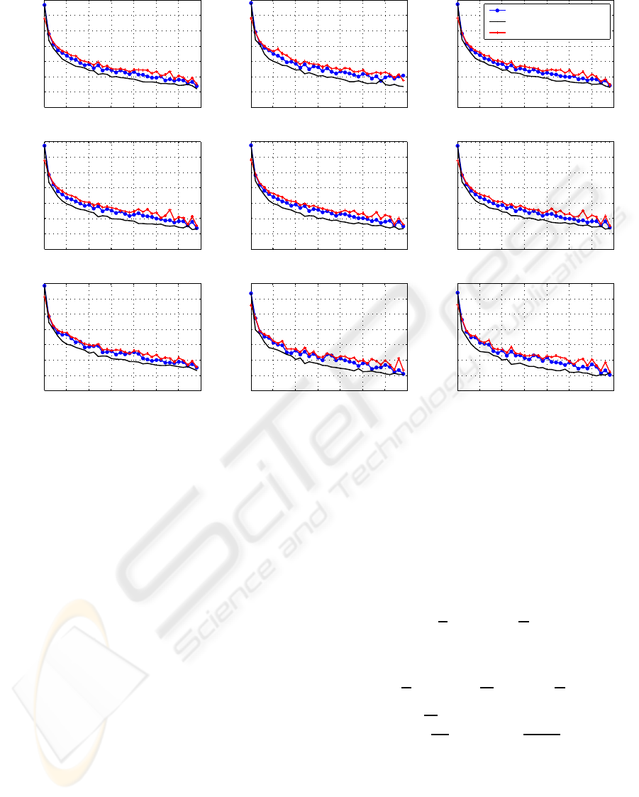
Figure 1: The averaged over 102 subjects MSD tracks provided by traditional averaging, weighted averaging and ERPSUB
(nine EEG channels, 30ms deviant, logarithmic scale).
subspaces orthogonal and standardize the data to sim-
ilar variances along all directions, and averaging ERP
components should have the largest variances in con-
trary to the noise components, and, hence, subspaces
can be extracted by standard linear Principal Com-
ponent Analysis (PCA) algorithm (Hyv¨arinen et al.,
2001; Oja, 1992). In practice, however, the variance
of data most likely will reduce along all directions af-
ter the averaging, because subspaces are overlapped,
and additive noise is always present, and, thus, pure
signal/noise subspaces do not exist. In this case the
results are interpreted in terms of SNR: higher SNR
is obtained in data projected to the directions describ-
ing larger data variations after whitening and aver-
aging. Thus, practically, we intend to separate the
subspace of dimension N
ERP
having maximal possi-
ble SNR from the subspace of dimension K − N
ERP
with the minimal possible SNR. As one can see, ERP-
SUB is based on a sequence of linear transformations
applied in a problem-specific manner to multidimen-
sional EEG data and results in effective denoising of
ERP signals (Ivannikov et al., 2007).
ERPSUB:
1. Whiten the centered concatenated data:
Z = D
−1/2
W
T
X, (21)
where matrices D andW are taken from the eigen-
value decomposition
b
Σ = WDW
T
of the estimated
covariance matrix
b
Σ = XX
T
/(TN − 1).
2. Average the whitened data:
Z = D
−1/2
W
T
X. (22)
3. Apply the standard linear PCA to the averaged
whitened data
Y
′
ERP
= ∆
N
ERP
W
T
D
−1/2
W
T
X, (23)
where matrix W
T
is obtained from the eigenvalue
decomposition ZZ
T
/(T − 1) = WDW
T
and ∆
N
ERP
is the diagonal projection matrix having ones on
N
ERP
first diagonal elements corresponding to the
components contributing energy to ERP (maximal
SNR) subspace and zeros otherwise. Here, N
ERP
is the amount of assumed ERP sources present in
EEG measurements. In practice, when pure sig-
nal/noise subspaces do not exist, N
ERP
has differ-
ent meaning interpreted in terms of SNR. In this
TRADITIONAL AVERAGING, WEIGHTED AVERAGING, AND ERPSUB FOR ERP DENOISING IN EEG DATA - A
Comparison of the Convergence Properties
199
50 100 150 200 250 300 350
10e−1
10e0
10e1
10e2
10e3
σ
n
2
, µV
2
C3
50 100 150 200 250 300 350
10e−1
10e0
10e1
10e2
10e3
C4
50 100 150 200 250 300 350
10e−1
10e0
10e1
10e2
10e3
Cz
50 100 150 200 250 300 350
10e−1
10e0
10e1
10e2
10e3
F3
50 100 150 200 250 300 350
10e−1
10e0
10e1
10e2
10e3
F4
50 100 150 200 250 300 350
10e−1
10e0
10e1
10e2
10e3
Fz
50 100 150 200 250 300 350
10e−1
10e0
10e1
10e2
10e3
N, number of trials
Pz
50 100 150 200 250 300 350
10e−1
10e0
10e1
10e2
10e3
N, number of trials
A1
50 100 150 200 250 300 350
10e−1
10e0
10e1
10e2
10e3
N, number of trials
A2
Conventional Average
Weighted Average
ERPSUB
<
−
σ
n
2
, µV
2
<
−
σ
n
2
, µV
2
−
<
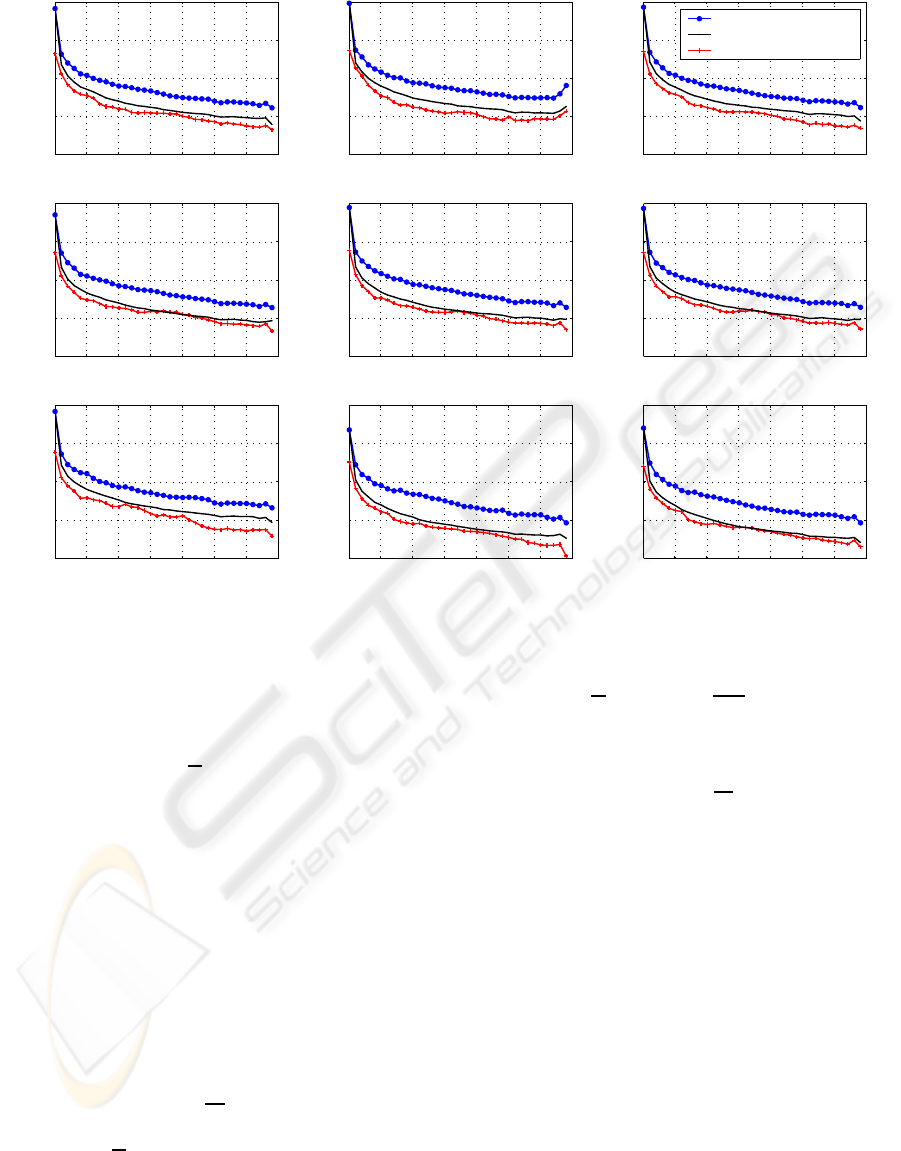
Figure 2: The averaged over 102 subjects tracks of the remaining noise variance in ERP estimates provided by traditional
averaging, weighted averaging and ERPSUB (nine EEG channels, 30ms deviant, logarithmic scale).
case N
ERP
is the amount of the components hav-
ing largest SNR, which in our opinion describe
ERP and noise variations in channels in propor-
tions providing suitable SNR and tolerable ERP
energy loss. Hence, Y
′
ERP
is a matrix of the av-
eraged components, where all components from
noise (minimal SNR) subspace are zeroed. Note
that ERP components have the largest correspond-
ing eigenvalues and, thus, the component classi-
fication problem is solved automatically for fixed
N
ERP
. In addition, if the difference between eigen-
values corresponding to ERP and noise compo-
nents is clearly observed, one can estimate N
ERP
value providing optimal separation of the compo-
nents into subspaces in the sense of SNR and ERP
energy loss. Moreover, each K-dimensional trial
X
i
can be decomposed into the components using
the same transformation as in (23):
Y
′
ERPi
= ∆
N
ERP
W
T
D
−1/2
W
T
X
i
, (24)
4. The matrix Y
′
ERP
containing only averaged com-
ponents related to ERP subspace is then trans-
formed back to the original data space (channels)
to result in the subject average with the reduced
noise:
X
ERP
= WD
1/2
WY
′
ERP
. (25)
A similar relation applies also to a single trial de-
noising:
X
ERPi
= WD
1/2
WY
′
ERPi
. (26)
4 EXPERIMENTAL RESULTS
It was noticed during the simulations and is theoreti-
cally predictable that the weighted averaging method
is highly sensitive to the trials having small portions
of variance concentrated on short time intervals. Gen-
erally, such trials do not carry much of the informa-
tion and are usually recorded at the saturation state of
the amplifier, when parts of the trials are truncated re-
sulting in peaks alternating with flat periods. Satura-
tion state occurs, when signal exceeds the dynamical
range of the amplifier. The weighting coefficients a
i
’s
assigned for such trials are very large following the al-
gorithm. As a consequence, when trials are weighted,
peaks in truncated trials become very strong against
a background of other trials’ amplitude resulting in a
BIOSIGNALS 2008 - International Conference on Bio-inspired Systems and Signal Processing
200

high frequency noise in the averaged signal. To an-
nul the harmful consequences introduced by the trun-
cated trials we performed the trial rejection procedure
for our data before doing the computations. The suc-
cessful upper limit of the trial’s variance for the trial
removal was 30µV
2
, which finally rejected all trun-
cated trials in our database.
Apparently, for our problem the converged ERP
estimate (subject average) is indicated by only in-
significant change introduced by the consequent trial.
We measure the amount of change between the two
subsequent ERP estimates in one channel for method
LABEL by MSD score:
MSD
LABEL
N
=
1
T
T
∑
t=1
(x
LABEL
N
(t) − x
LABEL
N−1
(t))
2
,
where x
LABEL
N
(t) denotes ERP estimate obtained after
application of a particular method LABEL involving
N trials. Thus, for example, for ERPSUB x
ERPSUB
N
(t)
equals to a rowin the matrix of averaged filtered chan-
nels X
ERP
corresponding to the considered channel;
for weighted averaging x
WA
N
(t) =
∑
N
i=1
ba
i
x
i
(t), where
ba
i
’s are computed as in (17) substituting approxima-
tion from (15) for σ
2
n
i
for all i = 1,... ,N. To compare
the convergence rates of ERP estimates provided by
methods under consideration at increase of the num-
ber of processed trials, we computed averaged over
102 subjects MSD values for N = 1,... ,350 (MSD
tracks) for each method (see Fig. 1). We did this
for the nine EEG channels and for 30ms deviant only,
where ERP appeared to be the strongest. The value
of N
ERP
parameter of ERPSUB method was set to 3,
that is, a good choice of maximal SNR subspace di-
mension for our data, because signal loss is insignif-
icant and noise reduction is sufficiently high result-
ing in essential SNR increase (Ivannikov et al., 2007).
According to the obtained results, the weighted av-
eraging procedure outperforms both the traditional
averaging scheme and ERPSUB algorithm, because
MSD provided by weighted averaging, in general, de-
creases faster than for other methods at increase of
the number of processed trials. The superiority of the
weighted averaging here is probably a consequence of
the core idea underlying the method. Weighted aver-
aging is designed in a way that trials are ’equalized’
in the sense of the variance. This should make the
convergence of the ERP estimate smoother and faster.
Although application of ERPSUB should result in
higher noise reduction rate than the conventional av-
erage provides (Ivannikov et al., 2007), ERPSUB
has shown the lowest convergence rate of MSD to
zero. Most likely this happens, because new-coming
trial influences the denoising of all previous trials by
changing the projection axes. Since the shapes of all
filtered trials are affected, when new trial is added to
processing, the difference between the two adjacent
ERP estimates becomes more significant.
Therefore, in order to have a complete and fair
comparative picture of the methods’ performance, we
also computed averaged over 102 subjects remaining
noise variances in ERP estimates obtained under the
same conditions as used in the first test (see Fig. 2).
We used the following estimate of the noise variance
in the averaged brain responses taken from (van de
Velde, 2000):
b
σ
2 LABEL
n
= var{
1
N
N
∑
i=1
(−1)
i
x
LABEL
i
(t)}, (27)
where x
LABEL
i
(t) is the modified trial x
i
(t) obtained
after application of method LABEL, and
b
σ
2 LABEL
n
is
the estimate of the remaining noise variance in ERP
estimate obtained after application of method LABEL
involving N trials. For instance, x
WA
i
(t) = ba
i
x
i
(t),
where ba
i
is computed as in (17) replacing σ
2
n
i
with
the approximation from (15) for all i = 1,. ..,N; and
x
ERPSUB
i
(t) equals to a row in the matrix of filtered
trial X
ERPi
corresponding to the considered channel.
In this test the performance order of the methods ap-
peared to be different. ERPSUB has shown now the
highest effectiveness in the sense of the noise reduc-
tion rate, since the remaining noise variance in ERP
estimate provided by ERPSUB, in general, decreased
faster than for other methods at increase of the num-
ber of processed trials. This outstanding performance
can be explained here by the algorithmic nature of
ERPSUB, which simultaneously operates through all
time, trial, and channel dimensions that allows more
efficient extraction of the information discriminating
ERP and noise from data. The conventional averag-
ing has shown the lowest noise reduction rate in ERP
estimate following the results of the test.
5 CONCLUSIONS
In this article we compared the performance of the
three methods used nowadays in EEG research for
ERP denoising: conventional averaging, weighted av-
eraging and ERPSUB. For this purpose we carried out
two tests investigating the convergence and the noise
reduction rates in ERP estimates provided by the se-
lected methods at increase of the number of processed
trials. The convergencerate of ERP estimate appeared
to be the highest for the weighted averaging technique
and the lowest for ERPSUB. However, ERPSUB has
shown stronger noise reduction power than the tra-
ditional and weighted averaging methods have. The
noise reduction rate in ERP estimate provided by the
TRADITIONAL AVERAGING, WEIGHTED AVERAGING, AND ERPSUB FOR ERP DENOISING IN EEG DATA - A
Comparison of the Convergence Properties
201

traditional averaging was the poorest among tested
methods.
The paper touches practical issues the neuropsy-
chology researchers are faced with during EEG/ERP
data processing and analyzing. Namely, it points out
the bottlenecks of the traditional averaging technique
used for the time-locked brain responses denoising.
The roots of these bottlenecks are connected to the
violation of the assumptions underlying the averag-
ing in real applications and insufficiently powerful
’decoding’ of the relevant information ’encrypted’ in
the data. The weighted averaging method addresses
the bottlenecks, which arise due to the violation of
the assumptions underlying traditional averaging. We
have shown that this strategy for improving the per-
formance and the reliability of the traditional averag-
ing technique can be derived based on different crite-
ria and, in particular, SNR and mean-square error as it
has been shown in (Hoke et al., 1984). ERPSUB tries
to eliminate the second type of the bottlenecks, which
come from the disability of the traditional averaging
to effectively extract from data the overall available
information related to ERP and noise discrimination.
ERPSUB ’decrypts’ more effectively this information
hidden in data, since it operates through all time, trial,
and channel dimensions.
REFERENCES
Davila, C. E. and Mobin, M. S. (1992). Weighted averaging
of evoked potentials. IEEE Transactions on Biomedi-
cal Engineering, 39(4):338–345.
Furst, M. and Blau, A. (1991). Optimal a posteriori time
domain filter for average evoked potentials. IEEE
Transactions on Biomedical Engineering, 38(9):827–
833.
Hoke, M., Ross, B., Wickesberg, R., and L¨utkenh¨oner, B.
(1984). Weighted averaging - theory and application
to electric response audiometry. Electroenceph. Clin.
Neurophysiol., 57:484–489.
Huttunen, T., Halonen, A., Kaartinen, J., and Lyytinen, H.
(2007). Does mismatch negativity show differences
in reading disabled children as compared to normal
children and children with attention deficit? Develop-
mental Neuropsychology, 31(3):453–470.
Hyv¨arinen, A., Karhunen, J., and Oja, E. (2001). Indepen-
dent component analysis. John Wiley & Sons, Inc.
Ivannikov, A., K¨arkk¨ainen, T., Ristaniemi, T., and Lyytinen,
H. (2007). Extraction of ERP from EEG data. In 9th
International Symposium on Signal Processing and its
Applications.
Jung, T.-P., Makeig, S., Humphries, C., Lee, T. W., McK-
eown, M. J., Iragui, V., and Sejnowski, T. (2000).
Removing electroencephalographic artifacts by blind
source separation. Psychophysiology, 37:163–178.
Kalyakin, I., Gonz´alez, N., Joutsensalo, J., Huttunen, T.,
Kaartinen, J., and Lyytinen, H. (2007). Optimal dig-
ital filtering versus difference waves on the mismatch
negativity in an uninterrupted sound paradigm. Devel-
opmental Neuropsychology, 31(3):429–452.
Łe¸ski, J. (2002). Robust weighted averaging. IEEE Trans-
actions on Biomedical Engineering, 49(8):796–804.
Łe¸ski, J. and Gacek, A. (2004). Computationally effective
algorithm for robust weighted averaging. IEEE Trans-
actions on Biomedical Engineering, 51(7):1280–
1284.
Luu, P., Tucker, D., and Makeig, S. (2004). Frontal mid-
line theta and the error-related negativity: neurophys-
iological mechanisms of action regulation. Clinical
Neurophysiology, 115(8):1821–35.
Makeig, S., Westerfield, M., Townsend, J., Jung, T.-P.,
Courchesne, E., and Sejnowski, T. (1999). Func-
tionally independent components of the early event-
related potentials in a visual spatial attention task.
Philosophical Transactions of the Royal Society B: Bi-
ological Sciences, 354:1135–44.
N¨a¨at¨anen, R. (1992). Attention and brain function.
Lawrence Erlbaum Associates, Hillsdale, New Jersey.
Oja, E. (1992). Principal components, minor components,
and linear neural networks. Neural Networks, 5:927–
935.
Pihko, E., Lepp¨asaari, T., and Lyytinen, H. (1995). Brain
reacts to occasional changes in duration of elements
in continues sound. NeuroReport, 6:1215–18.
van de Velde, M. (2000). Signal validation in electroen-
cephalography research. PhD thesis, Eindhoven Uni-
versity of Technology.
Vig´ario, R. (1997). Extraction of ocular artifacts from
EEG using independent component analysis. Elec-
troencephalography and Clinical Neurophysiology,
103:395–404.
BIOSIGNALS 2008 - International Conference on Bio-inspired Systems and Signal Processing
202
