
A NEW METHOD FOR THE DETECTION OF BRAIN STEM IN
TRANSCRANIAL ULTRASOUND IMAGES
Josef Schreiber
∗
, Eduard Sojka
∗
, La
ˇ
cezar Li
ˇ
cev
∗
, Petra
ˇ
Sk
ˇ
nou
ˇ
rilov
´
a
†
, Jan Gaura
∗
∗
Department of Computer Science,
†
Department of Applied Mathematics
V
ˇ
SB - Technical University of Ostrava, 17. listopadu 15/2172
Ostrava - Poruba, Czech Republic
David
ˇ
Skoloud
´
ık
Neurological clinic, Faculty Hospital in Ostrava-Poruba, 17.listopadu 1790, Ostrava - Poruba, Czech Republic
Keywords:
Ultrasound images, brain stem, detection, noise, speckle, Parkinson’s disease, object recognition.
Abstract:
Transcranial sonography is to date the only method able to detect structural damage of the brain tissue in the
Parkinson’s disease patients. The problem is that the images provided by this method often suffer from a
very poor quality, which makes the final diagnosis strongly dependent on experience of examinating medical
doctor. Our objective is to create a method that should help to minimize the physician’s subjectivity in the final
diagnosis and should provide more exact information about the processed ultrasound images. The method
itself is divided into two phases. In the first one, we try to locate the position of a minimal window containing
the brain stem in the analyzed image. In the second phase, we locate and measure the echogenic substantia
nigra area.
1 PARKINSON’S DISEASE
Parkinson’s disease (PD) belongs to the neurodegen-
erative diseases affecting mostly older people. It is a
chronic progressive disease that occurs if the nerve
cells in a part of the midbrain, called the substan-
tia nigra, die or are impaired. These nerve cells
produce dopamine, an important chemical messen-
ger that transmits signals from the substantia nigra to
other parts of the brain. These signals allow coordi-
nated movement. If the dopamine-secreting cells in
the substantia nigra die, the other movement control
centers in the brain become unregulated. Neuroimag-
ing methods are increasingly used as diagnostic tools
in patients presenting with parkinsonism. However,
brain computed tomography (CT) and magnetic res-
onance imaging (MRI) examinations are only able to
detect other aetiology than PD (Ressner, 2007). This
is why these traditional displaying methods like CT
and MRI are not considered to be conclusive (Bog-
dahn, 1998).
In 1995 Becker et al. published a study dealing
with the diagnostics of PD using transcranial sonog-
raphy (Becker, 1995). They showed that increased
echogenicity of substantia nigra is closely associated
with PD. Later, their research was followed by other
authors (Berg, 1999), (Berg, 2001). They proved that
hyperechogenic substantia nigra can be found in more
than 91% patients with PD. Nowadays the transcra-
nial sonography is considered to be the best possible
diagnostic tool for a detection of structural damage
of brain tissue in Parkinson’s disease patients. Ul-
trasonic imaging is based on detecting reflected and
scattered waves arising as a response to the emitted
wave with various frequencies. In general, the higher
the frequency is, the better and more detailed out-
put images can be obtained. Unfortunately, in the
case of transcranial sonography, we need to deal with
the scull that behaves as a barrier stopping all high-
frequency waves. This means that only the low fre-
quency probes (1-4 MHz) may be used. As a conse-
quence of this, transcranial sonography provides im-
ages of significantly lower quality (see Figure 1).
The interpretation of ultrasound images is gener-
ally a difficult task and the opinion of different med-
ical doctors is generally equivocal. The problem is
even more serious in transcranial sonography. Even if
the image is carefully evaluated by a physician, there
478
Schreiber J., Sojka E., Li
ˇ
cev L., Šk
ˇ
nourilová P., Gaura J. and Školoudík D. (2008).
A NEW METHOD FOR THE DETECTION OF BRAIN STEM IN TRANSCRANIAL ULTRASOUND IMAGES.
In Proceedings of the First International Conference on Bio-inspired Systems and Signal Processing, pages 478-483
DOI: 10.5220/0001057604780483
Copyright
c
SciTePress
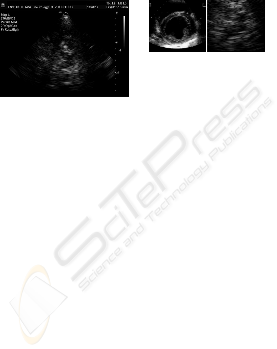
Figure 1: An example of processed sono image.
is a significant influence of subjectivity. By two dif-
ferent medical doctors, a different diagnosis may be
determined from one image. Another problem is a
long time treatment when the progress of the disease
must be determined from old images and repeating of
examination is no longer possible (
ˇ
Skoloud
´
ık, 2007).
That is why there appeared the demand to create a tool
that would help physicians to objectivize the diagno-
sis process. The processing of ultrasound images is
widely discussed in literature. Various methods were
presented for an image segmentation (Noble, 2006),
(Boukerroui, 2003), (Bosch, 2002), noise and speckle
reduction (Magnin, 1982), (Rakotomamonjy, 2000),
(Kerr, 1986) or image enhancement (Lee, 1980), (Sat-
tar, 1997). However, according to our knowledge,
there are no studies dealing with processing the brain-
stem transcranial images or with computerized recog-
nition of objects in the substantia nigra area.
Since the image segmentation is strongly depen-
dent on the character of the processed image we need
to realize that the usage of classic ultrasound image
segmentation methods will be limited. Still, some in-
teresting studies dealing with ultrasound images were
published. Ballard et al. (Ballard, 1982) presented
region-based segmentation methods such as the re-
gion growing where they used the homogeneity of
inner regions in the images. Such approach is ob-
viously impropriate for transcranial images process-
ing since the images contain too much ultrasound
speckle. Mishra et al. (Mishra, 2006) presented
the active contour method in combine with the ge-
netic algorithms for the endocardial border detection.
A slightly different approach was used by Mignotte
(Mignotte, 2001). They used a statistical external en-
ergy in a discrete active contour for the segmentation
of parasternal images. Their work was followed by
many optimization efforts, e.g., Heitz (Heitz, 1994).
The method provided relatively good results and is
recommended for the noisy ultrasound images. Still,
Figure 2: An endocardial (left) and transcranial (right )ul-
trasound image. The different level of noise is evident.
if we compare the level of noise in the images the
method was tested on with transcranial ultrasound im-
ages, we see that our analysed images have signifi-
cantly worse quality.
Another possible method for an ultrasound image
segmentation are the level sets, using an adaption of
the fast marching method. In 2003, Yan et al. (Yan,
2003) presented the purely edge-based version of this
method for the endocardial boundary detection. It was
later improved by Lin et al.(Lin, 2003). Their method
combined an edge and a region information in a level
set approach across spatial scales and it assumes that
a boundary is a closed curve. The method is supposed
to work well with the images of reasonably good qual-
ity. Klinger et al. (Klinger, 1988) presented a study
dealing with the echocardiographic images, based on
mathematical morphology. As well as the previous
method, this one also assumes to work with good
quality images. In 1999, Rekeczsky et al. (Rekeczky,
1999) and Binder et al. (Binder, 1999) came with the
artificial neural network method. Binder used a 2-
layer backpropagation network to identify a 7x7 pix-
els region with good results. Unfortunatly, we try to
locate a region 120x120 pixels large which means a
significant growth of input information for the neural
network. Even if we decide to use only some impor-
tant parts of the image to reduce the input, we still
have to deal with the possiblity that the selected re-
gion is strongly covered by ultrasound speckle. Our
proposed method is designed to use as much infor-
mation from analysed image as possible to avoid be-
ing misled by the high level of ultrasound noise and
speckle.
2 BRAIN STEM LOCALIZATION
The method we have developed for processing the
brain-stem transcranial sono images is divided into
two phases. In the first phase, we try to locate the
position of a minimal window in the processed im-
age containing the brain stem. To do so, we use a
modified template matching algorithm. Since every
human being is unique, the brain stems may slightly
A NEW METHOD FOR DETECTION OF BRAIN STEM IN TRANSCRANIAL ULTRASOUND IMAGES
479
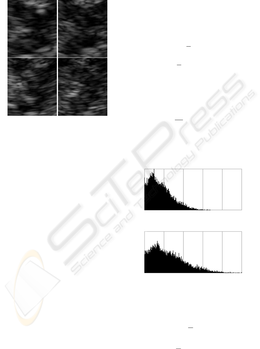
Figure 3: Examples of the images used for the template con-
struction. For need of this paper, the images are displayed
with the same size.
differ in shape and size. Moreover, the objects be-
ing sought inside the stem may have different posi-
tion, size, and echogenicity, depending on the disease
progress. Therefore, for creating the template of the
stem, we choose several images that best represent,
according to our opinion, various possible shapes and
sizes of the stem. We also consider the seriousness
of the disease by choosing images depicting the situa-
tion in various stages of the disease progress (from
healthy persons to persons with an advanced stage
of the disease). The selection of images that are
used for the template construction is important in
our method. Therefore, the selection of images was
widely discussed with medical doctors to best fulfill
previously mentioned parameters. Overall, there were
20 selected images used for the template construction.
Four examples of these images can be seen in Figure
3.
We construct the template that is used for match-
ing by simple averaging the particular selected images
of the brain stem. Firstly, the images are normalized
to the same size. In our experimental implementation,
we use the size of 120 × 120 pixels. After normaliz-
ing the size, we normalize the images of stem also
with respect to the mean value and the variance of
brightness. We do so by using the following formula
b
n
(x) = ab
o
(x) + c, (1)
where b
n
(x), b
o
(x) stand for the normalized and orig-
inal brightness, respectively, at a pixel whose position
is described by a two-dimensional vector x, and a and
c are constants that must be determined for each par-
ticular image. For determining them, the mean value
of brightness, denoted by µ
bo
, and the variance of
brightness, denoted by σ
2
bo
, in the original images are
needed. Let Ω stand for the set of all pixels in the
brain-stem image and let N be the size of this set. We
have
µ
bo
=
1
N
∑
x∈Ω
b
o
(x), (2)
σ
2
bo
=
1
N
∑
x∈Ω
(b
o
(x) − µ
bo
)
2
. (3)
In each normalized image, the normalization of
brightness aims at achieving a certain required mean
value, denoted by µ
bn
and a required variance of
brightness, denoted by σ
2
bn
. Simple mathematics
yields the following formulas for a and c
a =
σ
bn
σ
bo
, c = µ
bn
− aµ
bo
. (4)
The effect of normalization can be seen in Figures
4, 5. In Figure 6, the set of example images from Fig-
ure 3 can be seen in normalized form. An example of
the template that was obtained by averaging the brain-
stem images using Equation 5 is depicted in Figure 7.
Figure 4: The histogram of original image.
Figure 5: The histogram of normalized image.
In the pattern matching algorithm, we will also use
the variance of brightness in particular pixels that can
be expressed as follows
µ
b
(x) =
1
M
M
∑
j=1
b
n j
(x), (5)
σ
2
b
(x) =
1
M
M
∑
j=1
(b
n j
(x) − µ
b
(x))
2
. (6)
BIOSIGNALS 2008 - International Conference on Bio-inspired Systems and Signal Processing
480
Figure 6: The brain-stem images from Figure 3 after the
normalization process.
Figure 7: The constructed template.
In the above formulas, M is the number of partic-
ular normalized brain-stem images that are used for
creating the template; b
n j
stands for the j-th such im-
age.
In the first step of our method, we try to locate the
position of the brain stem. We introduce a possibil-
ity, denoted by π(u
k
, x), of the event that the template
point with the coordinates x corresponds to the image
point with the coordinates x + u
k
(Sojka, 2006). This
possibility may be determined from the difference of
brightness
∆b = b(x + u
k
) − t(x), (7)
where b(x +u
k
) is the brightness of the pixel with co-
ordinates x + u
k
in processed image, and t(x) is the
brightness in the corresponding template pixel. Let it
be pointed out that u
k
characterizes the template po-
sition that is just being processed.
We suppose that the possibility distribution may
be described by a certain chosen function ϕ. Figure
8 shows an example of such a function. For the con-
Figure 8: The distribution of possibility ϕ (we use the Gaus-
sian function).
struction of ϕ, we use the deviation σ
b
(x) that was
determined in Equation 6.
To obtain the possibility of the event that the im-
age pixel just being processed corresponds to the pixel
from the template, we use the following equation
π(u
k
, x) = ϕ(b(x + u
k
) − t(x), σ
b
(x)). (8)
To characterize the quality of matching at the po-
sition u
k
, we introduce the quantity S(u
k
) character-
izing the number of pixels, i.e., the ”net area” that can
successfully be matched to the template. We have
S(u
k
) =
∑
x∈Ω
π(u
k
, x), (9)
where Ω stands for the set of template pixels.
The final goal is to find the value of u that maxi-
mizes the value of S(u
k
). The value of u then deter-
mines the position of the window that should contain
the brain stem (Figure 9).
Figure 9: An image with the recognized brain-stem object.
It is obvious that during the brain-stem detec-
tion, each processed window from the analyzed image
must be normalized in the same way as the images
used for the template construction.
3 ANALYSIS OF BRAIN STEM
To obtain the information about the disease progress,
we now need to locate and measure the objects in-
side the brain stem, which is the second step of our
A NEW METHOD FOR DETECTION OF BRAIN STEM IN TRANSCRANIAL ULTRASOUND IMAGES
481
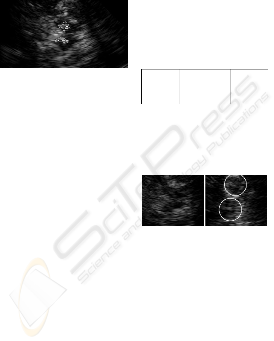
Figure 10: An image with the recognized brain stem and the
highlighted objects.
method. In the image, these objects appear as the
areas with a higher level of echogenicity inside the
substantia nigra area. It is a difficult task to correctly
identify these objects because the areas may have in-
sufficient contrast.
We locate the objects in the brain stem as the ar-
eas with a higher level of brightness that are found
using the region growing method. Homogenity of
brightness is a criterion that is used for growing. Af-
ter growing, the regions of interest are usually parti-
tioned into several smaller areas (Figure 10). There-
fore, morphological closing is carried out after grow-
ing to connect the sub-areas together. If it is required
by a doctor, the convex hull of the found area may
be computed too. The regions that have been found
are then checked for the shape and size, which sepa-
rates the objects of interest in the stem. The numerical
characteristics are then computed. For all recognized
objects, we determine the number of pixels the ob-
jects are composed of, their average brightness, and
the location of their gravity centers. Besides comput-
ing the characteristics of the objects, they can also be
highlighted in the images (Figure 10).
Naturally, there is also a possibility to correct the
obtained results manually, if necessary, and remove
possible unwanted objects that are considered to be
only a noise, ultrasound speckle or possibly even a
part that does not belong to the brain stem area.
4 ACHIEVED RESULTS
To test the succesfulness of our method in brain stem
localization, we used a sample of 170 images in which
we tried to locate the correct brain-stem position. The
result (the quality of recognition) was classified with
the marks between 1 and 3. The mark 1 means that the
position was recognized correctly and accurately. The
mark 2 means that the position was determined inac-
curately but not completely incorrectly. In this case,
the position was usually determined with an error up
to 10-15 pixels. The mark 3 means that the method
determined an incorrect position. For our set of test
images, we obtained the results that are summarized
in Table 1.
Table 1: The results of the brain-stem localization achieved
by the presented method. The first column determines the
quality of recognition. The second one shows the number of
images recognized with corresponding quality and the last
column displays the overall percentage.
Quality of
recognition
Number of images Results in %
1 129 75,9
2 4 2,3
3 37 21.8
The mark 1 was achieved in nearly 76% of
images. This can be considered as a good result since
we have to realize that the method must deal with
images of various quality. The difference between
the good and and bad image is shown in Figure 11.
In the left image, we can clearly see the shape of the
brain stem. For our method, the right image is very
difficult to determine the correct brain-stem location.
Figure 11: These images illustrate the difference between
the good quality and the bad quality images. While in the
left image, the shape and position of brain stem is obvious,
in the right image, two places with similar shape to the brain
stem may be found.
5 CONCLUSIONS
The computer processing of transcranial ultrasound
images is a complicated task. Images often suffer
from a very poor quality and they often have a high
level of noise and speckle. The objects that were rec-
ognized are often discontinuous, in worse cases even
incomplete. The objects inside the brain stem often
have insufficient contrast and they are usually frag-
mented by ultrasound speckle. Still, the objective
evaluation of these images can be very helpful in the
Parkinson disease diagnostics and treatment. It can
help the medical doctors to determine the correct di-
agnosis as well as the level of the disease progress.
BIOSIGNALS 2008 - International Conference on Bio-inspired Systems and Signal Processing
482

The exact and objective information about the ex-
amination from particular date can especially help in
longer time diagnostics when repeating of the exami-
nation is no longer possible.
Our method may be divided into two phases. At
first, it attempts to correctly identify the position of
brain stem in processed image. This phase is crucial
in overall diagnostics and this paper focuses mostly
on this part. In the second phase, we detect the ob-
jects of interest in the brain stem. The detection of
existence, shape, size, and echogenicity of these ob-
jects is a valuable contribution to the diagnostics of
Parkinson’s disease.
Achieved results obtained during testing make us
believe that the method we have developed for the de-
tection and analysis of the brain stem in transcranial
ultrasound images is successful. From the tested im-
ages, we obtained good results. In 76% of cases, the
position of the brain stem was correctly determined.
ACKNOWLEDGEMENTS
Presented results had been obtained during solving
the grant project code T401940412 supported by the
Academy of Sciences of the Czech Republic.
REFERENCES
Ballard, D.H., B. C. (1982). Computer vision. Prentice-
Hall, Englewood Cliffs, NJ.
Becker, G., B. U. G. C. e. a. (1995). Transcranial color-
coded real-time sonography of intracranial veins. nor-
mal values of blood flow velocities and findings in
superior sagittal sinus thrombosis. Journal of Neu-
roimaging, 5:87–94.
Berg, D., B. G. Z. B. T. O. H. E. e. a. (1999). Vulnerability
of the nigrostriatal system as detected by transcranial
ultrasound. Neurology, 53:1026–1031.
Berg, D., S. C. B. G. (2001). Echogenicity of the substantia
nigra in parkinson’s disease and its relation to clinical
findings. Journal of Neurology, 248:684–689.
Binder, T., S. M. M. D. S. H. B. T. M. G. P. G. (1999). Ar-
tificial neural networks and spatial temporal contour
linking for automated endocardial contour detection
on echocardiograms: A novel approach to determine
left ventricular contractile function. 25(7):1069–1076.
Bogdahn, U., B. G. S. F. (1998). Echoenhancers and tran-
scranial color duplex sonography. Blackwell Science,
Berlin.
Bosch, J.G., M. S. L. B. N. F. K. O. S. M. R. J. (2002). Au-
tomatic segmentation of echocardiographic sequences
by active appearance motion models. 21(11):1374–
1383.
Boukerroui, D., B. D. N. J. B. O. (2003). Segmentation
of ultrasound images - multiresolution 2d and 3d al-
gorithm based on global and local statistics. Pattern
Recognition Letters, 24(4-5):779–790.
Heitz, F., P. P. B. P. (1994). Multiscale minimization of
global energy functions in some visual recovery prob-
lems. 59:125–134.
Kerr, A.T., P. M. F. F. H. J. (1986). Speckle reduction in
pulse echo imaging using phase insensitive and phase
sensitive signal processing techniques. 8:11–28.
Klinger, J.W.J., V. C. F. T. A. L. T. (1988). Segmentation
of echocardiographic images using mathematical mor-
phology. 35(11):925–934.
Lee, J. (1980). Digital image enhancement and noise ltering
by use of local statistics. PAMI-2(2):165–168.
Lin, N., Y. W. D. J. (2003). Combinative multi-scale level
set framework for echocardiographic image segmen-
tation. 7(4):529–537.
Magnin, P.A., v. R. O. T. F. (1982). Frequency compound-
ing for speckle contrast reduction in phased array im-
ages. Ultrasonic Imaging, 4:267–281.
Mignotte, M., M. J. (2001). A multiscale optimization ap-
proach for the dynamic contour-based boundary de-
tection issue. 25(3):265–275.
Mishra, A., D. P. G. M. K. (2006). A ga based approach for
boundary detection of left ventricle with echocardio-
graphic image sequences. 21(11):967–976.
Noble, J.A., B. D. (2006). Ultrasound image segmentation:
A survey. IEEE Transactions on medical imagining,
25(8):987–1010.
Rakotomamonjy, A., D. P. M. P. (2000). Wavelet-based
speckle noise reduction in ultrasound b-scan images.
22:73–94.
Rekeczky, C., T. A. V. Z. R. T. (1999). Cnn-based spa-
tiotemporal nonlinear filtering and endocardial bound-
ary detection in echocardiography. 27(1):171–207.
Ressner, P., v. D. H. P. K. P. (2007). Hyperechogenicity of
the substantia nigra in parkinson’s disease. Journal of
Neuroimaging, 17(Issue 2):164–167.
Sattar, F., F. L. S. G. L. B. (1997). Image enhancement
based on nonlinear multi-scale method. 6:888–895.
Sojka, E. (2006). A motion estimation method based on
possibility theory. In Proceedings of IEEE ICIP, pages
1241–1244.
ˇ
Skoloud
´
ık, D., F. T. B. P. L. K. R. P. Z. O. H. P. H. R. K. P.
(2007). Reproducibility of sonographic measurement
of the substantia nigra. Ultrasound in Medicine & Bi-
ology, 33(9):1347–1352.
Yan, J.Y., Z. T. (2003). Applying improved fast marching
method to endocardial boundary detection in echocar-
diographic images. 24(15):2777–2784.
A NEW METHOD FOR DETECTION OF BRAIN STEM IN TRANSCRANIAL ULTRASOUND IMAGES
483
