
MOTION ESTIMATION IN MEDICAL IMAGE SEQUENCES USING
INVERSE POLYNOMIAL INTERPOLATION
Saleh Al-Takrouri
School of Electrical Engineering and Telecommunications, University of New South Wales, Sydney, NSW, Australia
and National ICT Australia Ltd, Sydney, NSW, Australia
Andrey V. Savkin
School of Electrical Engineering and Telecommunications, University of New South Wales, Sydney, NSW, Australia
Keywords:
Motion estimation, polynomial interpolation, inverse interpolation, medical image sequences.
Abstract:
We propose a new method for motion estimation between two successive frames in medical image sequences
and videos. The method is based on inverse polynomial interpolation.
1 INTRODUCTION
The applications of motion estimation have been in-
creasingly gaining interest in the field of medical
imaging. (Hemmendorff, 2001) proposed a frame-
work for motion estimation of 2D X-ray angiogra-
phy images and 3D MRI mammograms. Deformable
models were used by (Kurabayashi et al., 2005) to es-
timate the motion in time-series chest MR images.
(Auvray et al., 2006) applied motion estimation to
transparent X-ray image sequences.
Motion estimation is a key step in video cod-
ing and compression, which is an important tool to
achieve bandwidth reduction when transmitting med-
ical image sequences and videos. In addition, remote
and robot-assisted surgeries and medical diagnostic
tools can benefit from motion estimation in analyzing
and interpreting the motions of body parts.
2 PROBLEM STATEMENT
Consider the pair of images I
1
(r, c) and I
2
(r, c), both
of size R×C, where the spacial arguments r and c re-
fer to the pixel at the rth row and cth column. Here we
assume that the two images are successive frames in a
medical video or image sequence with spacial differ-
ences between the two images but no change in inten-
sity. The pixels I
2
(r, c) of the destination image can
be generated by shifting corresponding pixels in the
source image in the 2D space. Let τ
1
(r, c) and τ
2
(r, c)
be the horizontal and vertical shifts respectively, then
we can write
I
2
(r, c) = I
1
(r+ τ
2
(r, c), c+ τ
1
(r, c)) (1)
Sub-pixel shifts are approximated by 2D polynomial
interpolations within square neighborhoods of the
source image I
1
. The advantage of this choice is the
separability and simplicity of implementation that al-
lows an approximation of (1) to be written in an easily
manipulated form.
Now assume that |τ
1
(r, c)| ≤ p and |τ
2
(r, c)| ≤ p.
Then the neighborhood in consideration would be of
size (2p+ 1)× (2p+1) and the interpolation polyno-
mial is of order 2p. Define a vector function
u(τ
i
(r, c)) =
τ
2p
i
(r, c)
τ
2p−1
i
(r, c)
.
.
.
1
(2)
The polynomial approximation of (1) can be written
in the form
I
2
(r, c) = u
T
(τ
1
(r, c))A(r, c)u(τ
2
(r, c)) (3)
where A(r, c) is a (2p+ 1) × (2p + 1) matrix . For
simplicity, the spacial arguments (r, c) are dropped
from this point and assumed implicitly
I
2
= u
T
(τ
1
)Au(τ
2
) (4)
With τ
1
and τ
2
are the unknowns in equation (4),
our goal is to solve the inverse polynomial interpo-
lation problem represented by (4), which would also
solve the motion estimation problem described above.
212
Al-Takrouri S. and V. Savkin A. (2008).
MOTION ESTIMATION IN MEDICAL IMAGE SEQUENCES USING INVERSE POLYNOMIAL INTERPOLATION.
In Proceedings of the First International Conference on Bio-inspired Systems and Signal Processing, pages 212-215
DOI: 10.5220/0001057902120215
Copyright
c
SciTePress

Many motion estimation methods use multiscale
or hierarchial levels in order to process large motions,
the proposed method can handle the size of motions
that typically exist between two successive frames
and therefor we are not using any multiscale pyra-
mids.
3 POLYNOMIAL
INTERPOLATION
For a pixel that is assumed to move a maximum of
p pixels to the right or the left in a 1D source signal,
the neighborhood considered Y is of length 2p + 1
and centered at the element y(0). Using polynomial
interpolation, y(x) representing a shift from the center
by a value x where |x| ≤ p can be approximated by
using a polynomial of order 2p
y(x) = c
2p
x
2p
+ c
2p−1
x
2p−1
+ ··· + c
2
x
2
+ c
1
x+ c
0
(5)
The coefficients c
2p
···c
0
are found by solving a sys-
tem of 2p+ 1 linear equations of the form
XC = Y
T
(6)
where
X =
(−p)
2p
(−p)
2p−1
··· −p 1
(−p+ 1)
2p
(−p+ 1)
2p−1
··· −p+ 1 1
.
.
.
.
.
. ···
.
.
.
.
.
.
0 0 ··· 0 1
.
.
.
.
.
. ···
.
.
.
.
.
.
(p− 1)
2p
(p− 1)
2p−1
··· p− 1 1
p
2p
p
2p−1
··· p 1
C =
c
2p
c
2p−1
.
.
.
c
1
c
0
, Y
T
=
y(−p)
.
.
.
y(0)
.
.
.
y(p)
(7)
and the solution to the linear system is given by
C = QY
T
, Q = X
−1
(8)
The matrix X in (7) is a special form of the Van-
dermonde matrix. Its inverse can be found using an
explicit LU factorization discussed in the paper by
(Olver, 2006).
Denote the ith row of the matrix Q in (8) as q
i
.
The process of 1D polynomial interpolation can be
expressed as
y(x) = Y
2p+1
∑
i=1
q
T
i
x
i
(9)
The 1D polynomial interpolation in (9) can be ex-
tended to the 2D case. When a pixel in a 2D neigh-
borhood is assumed to move a maximum of p pixels
along any dimension, the neighborhood in considera-
tion is of size (2p+ 1) × (2p+ 1) and centered at the
pixel n(0, 0).
Recall that q
i
is the ith row of the matrix Q in (8).
We use the fact that the 2D polynomial interpolation
is separable to build the matrix A, with each element
on the ith row and jth column is given by
a
(i, j)
=
p
∑
m=−p
p
∑
n=−p
N(m, n)q
j
(m)q
i
(n) (10)
The process of 2D polynomial interpolation can be
expressed now as
I
2
=
2p+1
∑
i=1
2p+1
∑
j=1
a
(i, j)
τ
2p+1−i
1
τ
2p+1− j
2
(11)
with the matrix form of (11) is as given by (4).
4 SOLUTION OF INVERSE
INTERPOLATION
4.1 The Linear Approximation
First we start by finding a linear approximation of (4)
around some values
¯
τ
1
,
¯
τ
2
(to be defined later). The
first order approximation using Taylor series is easily
computed since the differentiation of (4) with respect
to ether τ
1
or τ
2
is trivial.
I
2
≈ u
T
(
¯
τ
1
)Au(
¯
τ
2
) +
˙
u
T
(
¯
τ
1
)Au(
¯
τ
2
)[τ
1
−
¯
τ
1
]
+u
T
(
¯
τ
1
)A
˙
u(
¯
τ
2
)[τ
2
−
¯
τ
2
]
(12)
Equation (12) is written in a form of a linear equa-
tion
¯
I(
¯
τ
τ
τ) = H(
¯
τ
τ
τ)τ
τ
τ (13)
where
¯
I(
¯
τ
τ
τ) = I
2
− u
T
(
¯
τ
1
)Au(
¯
τ
2
) + H(
¯
τ
τ
τ)
¯
τ
τ
τ
H(
¯
τ
τ
τ) =
˙
u
T
(
¯
τ
1
)Au(
¯
τ
2
) u
T
(
¯
τ
1
)A
˙
u(
¯
τ
2
)
¯
τ
τ
τ =
¯
τ
1
¯
τ
2
, τ
τ
τ =
τ
1
τ
2
(14)
An approximate solution to equation (13) can be
found as
τ
τ
τ = G(
¯
τ
τ
τ)
¯
I(
¯
τ
τ
τ)
G(
¯
τ
τ
τ) =
H
T
(
¯
τ
τ
τ)H(
¯
τ
τ
τ) + I
2
−1
H
T
(
¯
τ
τ
τ)
(15)
where I
2
is the 2× 2 identity matrix.
MOTION ESTIMATION IN MEDICAL IMAGE SEQUENCES USING INVERSE POLYNOMIAL INTERPOLATION
213

4.2 The Iterative Solution
Define
¯
τ
τ
τ(k) to be the accumulated shifts from initial
step until the kth step
¯
τ
τ
τ(k) =
k
∑
i=0
τ
τ
τ(i) (16)
Starting with an initial value
¯
τ
τ
τ(0) = 0, the linear equa-
tion (13) and its solution (15) can be used in an itera-
tive manner as follows
¯
τ
τ
τ(0) = 0
e(0) =
¯
I(
¯
τ
τ
τ(0))
τ
τ
τ(1) = G(
¯
τ
τ
τ(0))e(0)
= G(
¯
τ
τ
τ(0))
¯
I(
¯
τ
τ
τ(0))
e(1) =
¯
I(
¯
τ
τ
τ(1)) − H(
¯
τ
τ
τ(1))[τ
τ
τ(0) + τ
τ
τ(1)]
=
¯
I(
¯
τ
τ
τ(1)) − H(
¯
τ
τ
τ(1))
¯
τ
τ
τ(1)
τ
τ
τ(2) = G(
¯
τ
τ
τ(1))e(1)
= G(
¯
τ
τ
τ(1))[
¯
I(
¯
τ
τ
τ(1)) − H(
¯
τ
τ
τ(1))
¯
τ
τ
τ(1)]
.
.
.
(17)
In general
τ
τ
τ(k+ 1) = G(
¯
τ
τ
τ(k))[
¯
I(
¯
τ
τ
τ(k)) − H(
¯
τ
τ
τ(k))
¯
τ
τ
τ(k)] (18)
Substituting
¯
I(
¯
τ
τ
τ(k)) from equation (14) into equation
(18) yields the formula for the iterative numerical so-
lution as
τ
τ
τ(k+ 1) = G(
¯
τ
τ
τ(k))
I
2
− u
T
(
¯
τ
1
(k))Au(
¯
τ
2
(k))
(19)
When τ
τ
τ(k + 1) in the iterative equation (21) con-
verges to zero (or a small enough number near zero)
we get
¯
τ
τ
τ(k+ 1) such that
I
2
≃ u
T
(
¯
τ
1
(k+ 1))Au(
¯
τ
2
(k+ 1)) (20)
which is the solution to both problems of motion esti-
mation and inverse polynomial interpolation. Finally,
algebraic manipulation of (19) and using (16) sim-
plify the solution into the iterative formula given by
¯
τ
τ
τ(k+ 1) =
¯
τ
τ
τ(k) +
I
2
− u
T
(
¯
τ
1
(k))Au(
¯
τ
2
(k))
H(
¯
τ
τ
τ(k))H(
¯
τ
τ
τ(k))
T
H(
¯
τ
τ
τ(k))
T
(21)
Our solution in (21) is closely related to the al-
gorithm proposed by (Biemond et al., 1987). The
major difference is that in (Biemond et al., 1987) a
bilinear interpolation was used to calculate the dis-
placement frame difference, and the spatial gradients
were obtained by rounding off the displacement es-
timates; whereas in we use polynomial interpolation
which provides better interpolation and simplifies cal-
culating the gradients. Also, (Biemond et al., 1987)
used observations from a block of pixels.
Motion estimation results can be improved signif-
icantly by testing multiple initial values. Figure 1
Figure 1: The circled pixel positions are the chosen initial
positions for the 5× 5 neighborhood.
shows the chosen initial positions for the 5× 5 neigh-
borhood (i.e. p = 2). For the (2p + 1) × (2p + 1)
neighborhood, the number of initial values
¯
τ
τ
τ(0) is p
2
.
The different initial values are sorted and tried accord-
ing to their distance from the mean shift obtained for
the previously processed adjacent pixels in I
2
, starting
with the closest. This also establishes dependency be-
tween the motions of the image pixels. For an initial
value, if the iterative equation (21) converges to a so-
lution before reaching a specified maximum number
of iterations, the result is recorded and there would be
no need to try the other initial values. Otherwise, the
next initial value is tried.
5 RESULTS
We tested our method using gray-scaled images. For
comparison, motion in the same frames was estimated
by the elastic image registration method by (Peri-
aswamy and Farid, 2003) and the widely-used optical
flow method by (Lucas and Kanade, 1981). The Mat-
lab code for Periaswamy and Farid’s method is avail-
able on the internet (Web, 1). Examples show that our
method provides better performance.
In the first example (Figure 2) two images are
extracted from an echocardiography video (Web, 2).
The images are of size 430× 550 pixels. The second
example (Figure 3) shows two images extracted from
a video recorded during a robotic-assisted repair of a
pulmonary artery (Web, 3). The images are of size
240× 352 pixels. For both examples we chose p = 7,
a convergence threshold of 0.001 and the maximum
number of iterations to be 20.
For each example, we computed the peak signal-
to-noise ratio (PSNR) for the displaced frame differ-
ence. The PSNR equation is defined by (22) and the
results are listed in Table 1.
PSRN = 10log
10
255
2
RC
R
∑
r=1
C
∑
c=1
(I
2
(r, c) − I
s
(r, c))
2
(22)
BIOSIGNALS 2008 - International Conference on Bio-inspired Systems and Signal Processing
214
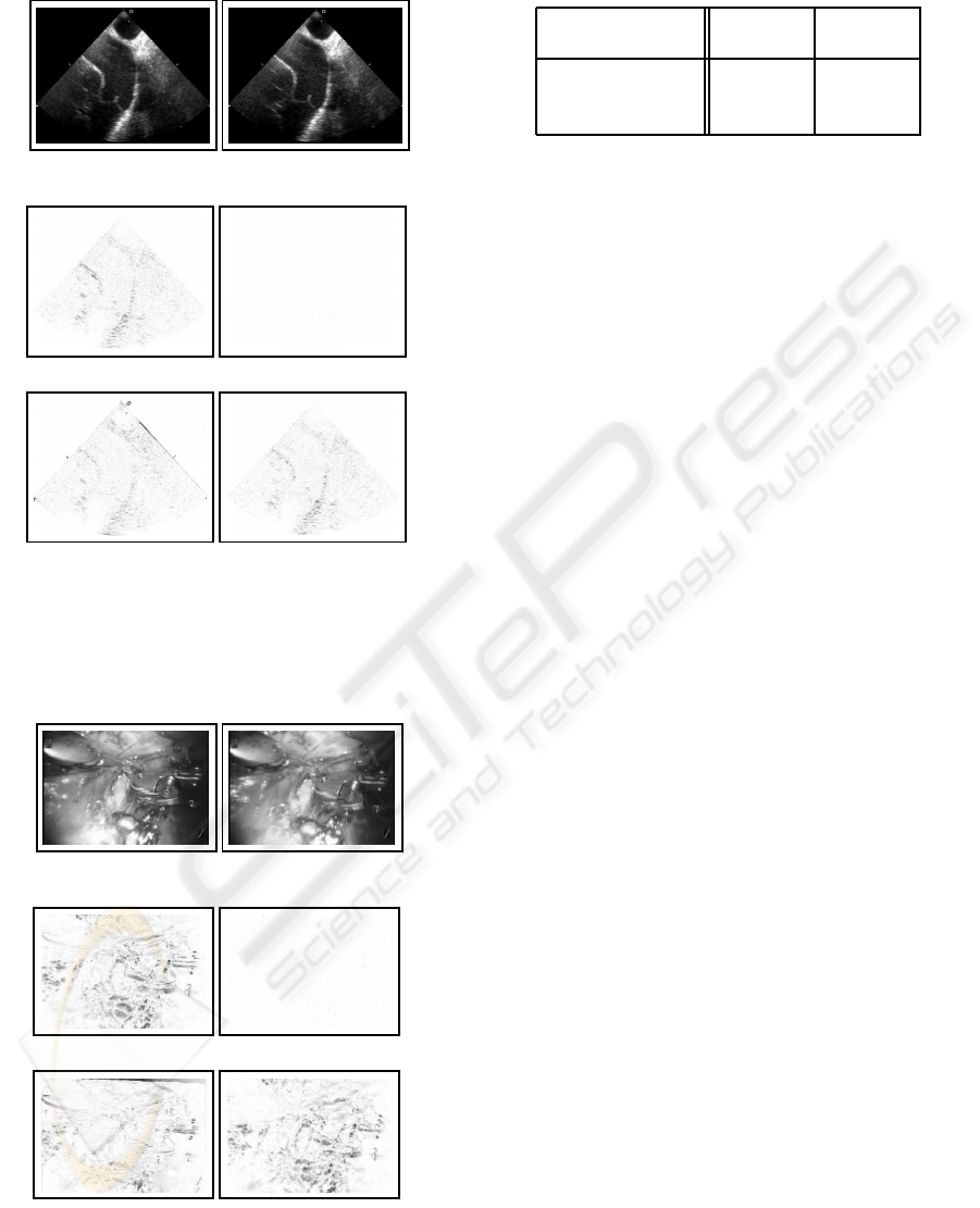
(a) Source image I
1
(b) Destination image
I
2
(c) |I
2
− I
1
| (d) |I
2
− I
AS
|
(e) |I
2
− I
PF
| (f) |I
2
− I
LK
|
Figure 2: Motion estimation between two successive frames
from echocardiography video.
(a) Source image I
1
(b) Destination image
I
2
(c) |I
2
− I
1
| (d) |I
2
− I
AS
|
(e) |I
2
− I
PF
| (f) |I
2
− I
LK
|
Figure 3: Motion estimation between two successive frames
from robot-assisted artery surgery video.
Table 1: PSNR of displaced frame difference.
Echocar- Artery
diography Surgery
Our method 50.27 dB 42.34 dB
Periaswamy-Farid 25.66 dB 19.85 dB
Lucas-Kanade 27.10 dB 19.12 dB
In (Periaswamy and Farid, 2003) the motion
within a small neighborhood was modeled locally by
an affine transform. In video sequences the consid-
ered neighborhood may contain one or more different
motions in addition to the stationary background. An
attempt to model these motions and the static back-
ground using one affine transform will produce esti-
mation errors. Our method does not suffer from this
shortcoming because it works on a pixel level.
ACKNOWLEDGEMENTS
This work was supported by National ICT Australia
and the Australian Research Council.
REFERENCES
Auvray, V., Bouthemy, P., and Lienard, J. (2006). Mo-
tion estimation in x-ray image sequences with bi-
distributed transparency. In Proceedings of the IEEE
International Conference on Image Processing, pages
1057–1060.
Biemond, J., Looijenga, L., Boekee, D., and Plompen, R.
(1987). A pel-recursive wiener-based displacement
estimation algorithm. Signal Processing, pages 399–
412.
Hemmendorff, M. (2001). Motion estimation and compen-
sation in medical imaging. PhD Thesis, Linkopings
University, Sweden.
Kurabayashi, Y., Kagei, S., Gotoh, T., and Iwasawa, T.
(2005). Motion estimation for sequential medical im-
ages using a deformable model. Systems and Comput-
ers in Japan, 36:27–36.
Lucas, B. and Kanade, T. (1981). An iterative image regis-
tration technique with an application to stereo vision.
In Proceedings of the DARPA Image Understanding
Workshop, pages 121–130.
Olver, P. (2006). On multivariant interpolation. Studies in
Applied Mathematics, 116:201–240.
Periaswamy, S. and Farid, H. (2003). Elastic registration
in the presence of intensity variations. IEEE Transac-
tions on Medical Imaging, 22:865–874.
Web (1). http://www.cs.dartmouth.edu/farid/research/.
Web (2). http://www.cts.usc.edu/videos.html.
Web (3). http://www.manbit.com/ers/ersvideo.asp.
MOTION ESTIMATION IN MEDICAL IMAGE SEQUENCES USING INVERSE POLYNOMIAL INTERPOLATION
215
