
AN EFFICIENT METHOD FOR VESSEL WIDTH MEASUREMENT
ON COLOR RETINAL IMAGES
Alauddin Bhuiyan, Baikunth Nath, Joselito Chua and Kotagiri Ramamohanarao
Department of Computer Science and Software Engineering and NICTA Victoria Research Laboratory
The University of Melbourne, Australia
Keywords:
Microvascular Sign, Gradient Operator, Adaptive Region Growing Technique, Texture Classification, Gabor
Energy Filter Bank, Fuzzy C-Means Clustering.
Abstract:
Vessel diameter is an important factor for indicating retinal microvascular signs. In automated retinal image
analysis, the measurement of vascular width is a complicated process as most of the vessels are few pixels
wide. In this paper, we propose a new technique to measure the retinal blood vessel diameter which can be
used to detect arteriolar narrowing, arteriovenous (AV) nicking, branching coefficients, etc. to diagnose related
diseases. First, we apply the Adaptive Region Growing (ARG) segmentation technique to obtain the edges
of the blood vessels. Following that we apply the unsupervised texture classification method to segment the
blood vessels from where we obtain the vessel centreline. Then we utilize the edge image and vessel centreline
image to obtain the potential pixels pairs which pass through a centreline pixel. We apply a rotational invariant
mask to search the pixel pairs from the edge image. From those pixels we calculate the shortest distance pair
which will be the vessel width for that cross-section. We evaluate our technique with manually measured
width for different vessels’ cross-sectional area and achieve an average accuracy of 95.8%.
1 INTRODUCTION
Accurate measurement of retinal vessel diameter is
an important part in the diagnosis of many diseases.
A variety of morphological changes occur to retinal
vessels in different disease conditions. The change
in width of retinal vessels within the fundus image is
believed to be indicative of the risk level of diabetic
retinopathy; venous beading (unusual variations in di-
ameter along a vein) is one of the most powerful pre-
dictor of proliferate diabetic retinopathy. Generalized
and focal retinal arteriolar narrowing and arteriove-
nous nicking have been shown to be strongly associ-
ated with current and past hypertension reflecting the
transient and persistent structural effects of elevated
blood pressure on the retinal vascular network. In
addition, retinal arteriolar bifurcation diameter expo-
nents have been shown to change significantly in pa-
tients with peripheral vascular disease and arterioscle-
rosis and a variety of retinal microvascular abnormal-
ities have been shown to relate to the risk of stroke
(Lowell et al., 2004). Therefore, an accurate measure-
ment of vessel diameter and geometry is necessary for
effective diagnosis of such diseases.
The measurement of the vascular diameter is crit-
ical and a challenging task whose accuracy depends
on the accuracy of the segmentation method. A re-
view for the blood vessel segmentation is provided in
the literature (Bhuiyan et al., 2007a). The study of
vessel diameter measurement is still an open area for
improvement. Zhou et al. (Zhou et al., 1994) have
applied a model-based approach for tracking and to
estimating widths of retinal vessels. Their model as-
sumes that image intensity as a function of distance
across the vessel displays a single Gaussian form.
However, high resolution fundus photographs often
display a central light reflex (Brinchman-hansan and
Heier, 1986). Intensity distribution curves is not al-
ways of single Gaussian form, so that using a sin-
gle Gaussian model for simulating intensity profile
of vessel could produce poor fits and subsequently
provide inaccurate diameter estimations (Gao et al.,
2001). Gao et al. (Gao et al., 2001) model the in-
tensity profiles over vessel cross section using twin
Gaussian functions to acquire vessel width. This tech-
nique may produce poor results in case of minor ves-
sels where the contrast is less. Lowell et al. (Low-
ell et al., 2004) have proposed an algorithm based on
fitting a local 2D vessel model, which can measure
vascular width to an accuracy of about one third of
178
Bhuiyan A., Nath B., Chua J. and Ramamohanarao K. (2008).
AN EFFICIENT METHOD FOR VESSEL WIDTH MEASUREMENT ON COLOR RETINAL IMAGES.
In Proceedings of the First International Conference on Bio-inspired Systems and Signal Processing, pages 178-185
DOI: 10.5220/0001059401780185
Copyright
c
SciTePress
a pixel. However, the technique is biased on smooth
data (image) and suffers from measuring the width of
minor vessels where the contrast is very less.
In this paper, we introduce a new algorithm, based
on vessel centreline and edges information. We ap-
ply the adaptive region growing technique to segment
the vessels edges (Bhuiyan et al., 2007a) and the un-
supervised texture classification method to segment
the vessels and detect the centreline (Bhuiyan et al.,
2007b). For each selected centerline pixel we map the
edge image of the retinal vessels edge pixels and find
all the potential line end points or pairing pixels on
opposite edge passing through this centreline pixels.
From these potential lines we find the line that has the
minimum length and consider this as the vessel width
for that cross-sectional area. In this way, we can mea-
sure the width of the blood vessel continuing through
the centreline of all the vessels. A specific feature of
our technique is that it can calculate the vessel width
when it is one pixel wide.
The rest of the paper is organized as follows: Sec-
tion 2 introduces the proposed method of blood ves-
sel width measurement. Edge based blood vessel seg-
mentation technique is described in section 3. Section
4 illustrates the vessel centreline detection procedure.
The vessel width measurement method is described
in section 5. The experimental results are provided
in section 6 and finally the conclusion and future re-
search directions are drawn in section 7
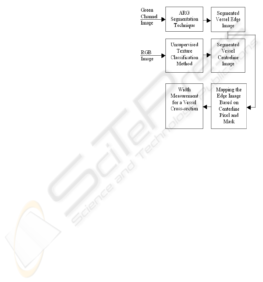
2 PROPOSED METHOD
We propose the blood vessels’ width measurement al-
gorithm based on the vessel edge and centreline. The
major advantage of our technique is that it is less sen-
sitive to noise and work equally for the low contrast
vessels (particularly for minor vessels). We adopt two
segmented images that are produced from the original
RGB image. At first, we apply the ARG segmenta-
tion technique to obtain the vessel edges, then we ap-
ply the unsupervised texture classification method to
segment the blood vessels from where we obtain the
vessel centreline. We map the vessel centreline image
and pick any of the vessel centreline pixel. For that
particular pixel we apply a rotational invariant mask
whose centre is that pixels position and searches the
potential pixels from the edge image using a contin-
uous increment of lower to higher distance and ori-
entation. For each case, if the gray scale value of that
pixel position is 255 or white it finds the mirror of this
pixel by searching through a fixed angle (exactly in-
crementing 180 degree) but in variable distance. This
is to give the flexibility and consistency to our method
as the centreline pixels may not be in the exact posi-
tion of vessel centre. In this way, we can obtain all the
potential pairs (line end points) which pass through
that centreline pixel. From those pairs we calculate
the minimum distance/length pair which is the width
of that cross-section of the blood vessel. Figure 1 de-
picts the overall technique of our proposed method.
Figure 1: The overall system for measuring blood vessel
width.
3 VESSEL EDGE DETECTION
We implemented the vessel segmentation technique
based on vessel edges. In the following subsections
we provide a brief illustration of this method.
3.1 Preprocessing of Retinal Image
Adaptive Histogram Equalization (AHE) method is
implemented, using MATLAB, to enhance the con-
trast of the image intensity by transforming the val-
ues using contrast-limited adaptive histogram equal-
ization (Figure 2).
3.2 Image Conversion
The enhanced retinal image is converted into gradient
image (Figure 2) using first order partial differential
operator. The gradient of an image f(x,y) at location
(x,y) is defined as the two dimensional vector (Gon-
AN EFFICIENT METHOD FOR VESSEL WIDTH MEASUREMENT ON COLOR RETINAL IMAGES
179
zalez and Wintz 1987)
G[ f(x, y)] = [G
x
,G
y
] =
∂f
∂x
,
∂f
∂y
(1)
For edge detection, we are interested in the magni-
tude G[ f(x,y)] and direction α(x,y)of the vector, gen-
erally referred to simply as the gradient and denoted
and commonly takes the value of
G[ f(x, y)] ≈ |G
x
| + |G
y
|
α(x,y) = tan
−1
(G
y
/G
x
)
(2)
where the angle is measured with respect to the x axis.
Figure 2: Original retinal image, its Adaptive Histogram
Equalized image (top; left to right), the Gradient Image and
final ARG output image (bottom; left to right).
3.3 Adaptive Region Growing
Technique
The edges of vessels are segmented using region
growing procedure(Gonzalez et al., 2004) that groups
pixels or sub regions into larger regions based on gra-
dient magnitude. As the gradient magnitude is not
constant for the whole vessel we need to consider an
adaptive gradient value that gradually increases or de-
creases to append the pixel to a region. We call it an
adaptive procedure, as the difference of neighboring
pixels intensity value is always adapted for the region
growing process. The region growing process starts
with appending the pixels that pass certain threshold
value. For region growing we find the intensity dif-
ference between a pixel belonging to a region and
its neighboring potential region growing pixels. The
pixel is considered for appending in that region if the
difference is less than a threshold value. The thresh-
old value is calculated by considering the maximum
differential gradient magnitude for any neighboring
pixels with equal (approximately) gradient direction.
Region growing should stop when no more pixels sat-
isfy the criteria for inclusion in that region. In the
region growing process each region is labeled with a
unique number. For that purpose we construct a cell
array with region number and its pixel position. The
image is scanned in a row-wise manner until its end,
and each pixel that satisfies our criteria is taken into
account for growing a region with its 8-neighborhood
connectivity.
3.4 Parallel Region Detection
We calculate the parallel edges (regions) by consid-
ering pixel orientation belonging to each region. At
first, we pick the region number and belonging pixel
coordinates from the constructed cell array. Then we
grouped the region/regions parallel to each region,
which is calculated by mapping the pixels gradient
direction. For each region every pixel is searched
from its potential parallel region and once a maximum
number of pixels match with the other region we con-
sider it as parallel to that region. We consider all re-
gions and once a region is considered we assigned a
flag value to that region so that it will not be consid-
ered again. In this way we can only filter the vessels
from the region and discard all other regions, which
are background noise or other objects like haemor-
rhage, macula, etc in the retinal image.
3.5 Experimental Results
We considered DRIVE database (DRIVE-database,
2004) and applied our technique on five images for
initial assessment. For performance evaluation we
employed an expert to find the number of vessels in
the original image and detected output image (Figure
2). We achieved an overall 94.98% detection accu-
racy.
4 VESSEL CENTRELINE
DETECTION
We implemented the unsupervised texture classifica-
tion based vessel segmentation method from which
we detect the vessel centreline. We consider Gaus-
sian and L
∗
a
∗
b
∗
perceptually uniform color spaces
with the original RGB image for texture feature ex-
traction. To extract features, a bank of Gabor energy
filters with three wavelengths and twenty-four orien-
tations is applied in each selected color channel. Then
BIOSIGNALS 2008 - International Conference on Bio-inspired Systems and Signal Processing
180
a texture image is constructed from the maximum re-
sponse of all orientations for a particular wavelength
in each color channel. From the texture images, a fea-
ture vector is constructed for each pixel. These fea-
ture vectors are classified using the Fuzzy C-Means
(FCM) clustering algorithm. Finally, we segment the
image based on the cluster centroid value.
4.1 Color Space Transformation and
Preprocessing
Generally image data is given in RGB space (because
of the availability of data produced by the camera
apparatus). The definition of L
∗
a
∗
b
∗
is based on an
intermediate system, known as the CIE XYZ space
(ITU-Rec 709). This space is derived from RGB as
below (Wyszecki and Stiles, 1982)
X = 0.412453R + 0.357580G+ 0.180423B
Y = 0.212671R+ 0.715160G+ 0.072169B
Z = 0.019334R+ 0.119193G+ 0.950227B
(3)
L
∗
a
∗
b
∗
color space is defined as follows:
L
∗
= 116f(Y/Y
n
) − 16
a
∗
= 500[ f(X/X
n
) − f(Y/Y
n
)]
b
∗
= 200[ f(Y/Y
n
)] − f(Z/Z
n
)
(4)
where f(q) = q
1/3
if q < 0.008856 and is constant
7.87+16/116 otherwise. X
n
, Y
n
and Z
n
represent a
reference white as defined by a CIE standard illumi-
nant, D
65
in this case. This is obtained by setting
R = G = B = 100 in (1), q ∈ {X/X
n
,Y/Y
n
,Z/Z
n
}.
Gaussian color model can also be well approxi-
mated by the RGB values. The first three components
ˆ
E,
ˆ
E
λ
and
ˆ
E
λλ
of the Gaussian color model (Taylor
expansion of the Gaussian weighted spectral energy
distribution at Gaussian central wavelength and scale)
can be approximated from the CIE 1964 XYZ ba-
sis when taking λ
0
= 520nm (Gaussian central wave-
length) and σ
λ
= 55nm (scale) as follows (Geuse-
broek et al., 2001)
ˆ
E
ˆ
E
λ
ˆ
E
λλ
=
−0.48 1.2 0.28
0.48 −0.4 −0.4
1.18 −1.3 0
X
Y
Z
(5)
The product of (3) and (5) gives the desired imple-
mentation of the Gaussian color model in RGB terms
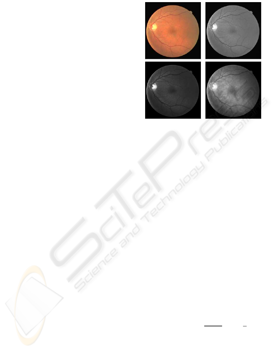
(Figure 3). The Adaptive Histogram Equalization
method was implemented, using MATLAB, to en-
hance the contrast of the image intensity.
4.2 Texture Feature Extraction
Texture generally describes second order property of
surfaces and scenes, measured over image intensities.
Figure 3: Original RGB and its Green channel image (top;
left to right), Gaussian transformed first and second compo-
nent image (bottom; left to right).
A Gabor filter has weak responses along all orien-
tations on the smooth (background) surface. On the
other hand, when it positioned on a linear pattern ob-
ject (like a vessel) the Gabor filter produces relatively
large differences in its responses when the orientation
parameter changes (Wu et al., 2006). Hence, the use
of Gabor filters to analyze the texture of the retinal
images is very promising. In the following two sub-
sections we illustrate the Gabor filter based texture
analysis method.
4.2.1 Gabor Filter
An input image I(x,y), (x,y) ∈ Ω where Ω is the set of
image points, is convolved with a 2D Gabor function
g(x,y), (x,y) ∈ ω, to obtain a Gabor feature image
r(x, y) (Gabor filter response) as follows (Kruizinga
and Petkov, 1999)
r(x, y) =
ZZ
Ω
I(ξ, η)g(x− ξ,y− η)dξdη (6)
We use the following family of 2D Gabor functions to
model the spatial summation properties of an image
(Kruizinga and Petkov, 1999)
g
ξ,η,λ,Θ,φ
(x,y) = exp(−
x
′2
+γ
2
y
′2
2σ
2
)cos(2π
x
′
λ
+ φ)
x
′
= (x− ξ) cosΘ− (y− η)sinΘ
y
′
= (x− ξ) cosΘ− (y− η)sinΘ
(7)
where the arguments x and y specify the position of
a light impulse in the visual field and ξ,η,σ,γ, λ,Θ,φ
are parameters. The pair (ξ,η) specifies the center of
a receptive field in image coordinates. The standard
AN EFFICIENT METHOD FOR VESSEL WIDTH MEASUREMENT ON COLOR RETINAL IMAGES
181
deviation σ of the Gaussian factor determines the size
of the receptive filed. Its eccentricity is determined by
the parameter γ called the spatial aspect ratio. The pa-
rameter λ is the wavelength of the cosine factor which
determines the preferred spatial frequency
1
λ
of the
receptive field function g
ξ,η,λ,Θ,φ
(x,y). The parame-
ter Θ specifies the orientation of the normal to the
parallel excitatory and inhibitory stripe zones - this
normal is the axis x
′
in (5). Finally, the parameter
φ ∈ (−π,π), which is a phase offset argument of the
harmonic factor cos(2π
x
′
λ
+ φ), determines the sym-
metry of the function g
ξ,η,λ,Θ,φ
(x,y).
4.2.2 Gabor Energy Features
A set of textures was obtained based on the use of
Gabor filters (6) according to a multichannel filter-
ing scheme. For this purpose, each image was filtered
with a set of Gabor filters with different preferred ori-
entation, spatial frequencies and phases. The filter re-
sults of the phase pairs were combined, yielding the
Gabor energy quantity (Kruizinga and Petkov, 1999):
E
ξ,η,Θ,λ
=
q
r
2
ξ,η,Θ,λ,0
+ r
2
ξ,η,Θ,λ,π/2
(8)
where r
2
ξ,η,Θ,λ,0
and r
2
ξ,η,Θ,λ,π/2
are the outputs of the
symmetric and antisymmetric filters. We used Gabor
energy filters with twenty-four equidistant preferred
orientations(Θ = 0,15,30, ..,345) and three preferred
spatial frequencies (λ = 6,7,8). In this way an ap-
propriate coverage was performed of the spatial fre-
quency domain.
We considered the maximum response value per
pixel on each color channel to reduce the feature vec-
tor length and complexity of training on data for the
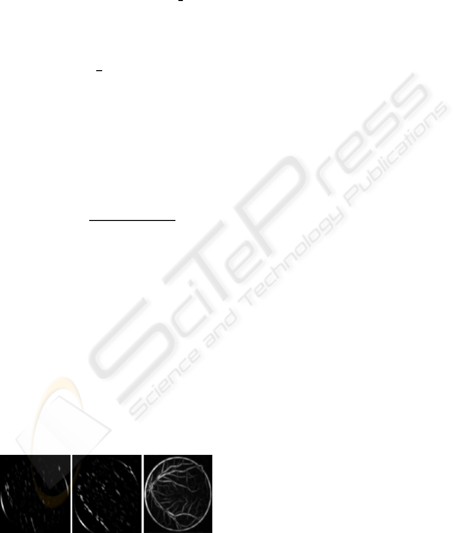
classifier. In addition, we constructed an image (Fig-
ure 4) on each color channel which was used for
histogram analysis to determine the cluster number.
From these images we constructed twelve element
length feature vector for each pixel in each retinal im-
age to classify them into vessel and non-vessel using
the FCM clustering algorithm.
Figure 4: Texture analyzed image with the orientations of
15, 45 degrees and maximum response of all twenty-four
orientations (left to right).
4.3 Texture Classification and Image
Segmentation
The FCM is a data clustering technique where in each
data point belongs to a cluster to some degree that is
specified by a membership grade. Let X = x
1
,x
2
,,x
N
where x ∈ R
N
present a given set of feature data. The
objective of the FCM clustering algorithm is to mini-
mize the Fuzzy C-Means cost function formulated as
(Bezdek, 1981)
J(U,V) =
C
∑
j=1
N
∑
i=1
(µ
ij
)
m
||x
i
− v
j
||
2
(9)
V = {v
1
,v
2
,,v
C
} are the cluster centers. U = (µ
ij
)
N×C
is fuzzy partition matrix, in which each member is be-
tween the data vector x
i
and the cluster j. The values
of matrix U should satisfy the following conditions:
µ
ij
∈ [0,1], i = 1, ..,N, j = 1, ..,C (10)
µ
ij
= 1,i = 1,.., N (11)
The exponent m ∈ [1,∞] is the weighting exponent,
which determines the fuzziness of the clusters. The
most commonly used distance norm is the Euclidean
distance d
ij
= ||x
i
− v
j
||.
We used the Matlab Fuzzy Logic Toolbox for clus-
tering 253440 vectors (the size of the retinal image is
512x495) in length twelve for each retinal image. In
each retinal image clustering procedure, the number
of clusters was assigned after analyzing the histogram
of the texture image. The parameter values used for
the FCM clustering were as follows. The exponent
value of 2 for the partition matrix, maximum number
of iterations was set to 1000 for the stopping crite-
rion and the minimum amount of improvement be-
ing 0.00001. We received the membership values on
each cluster for every vector, from which we picked
the cluster number that belonged to the highest mem-
bership value for each vector and converted it into a
2D matrix. From this matrix we produced the binary
image considering the cluster central intensity value
which identifies the blood vessels only.
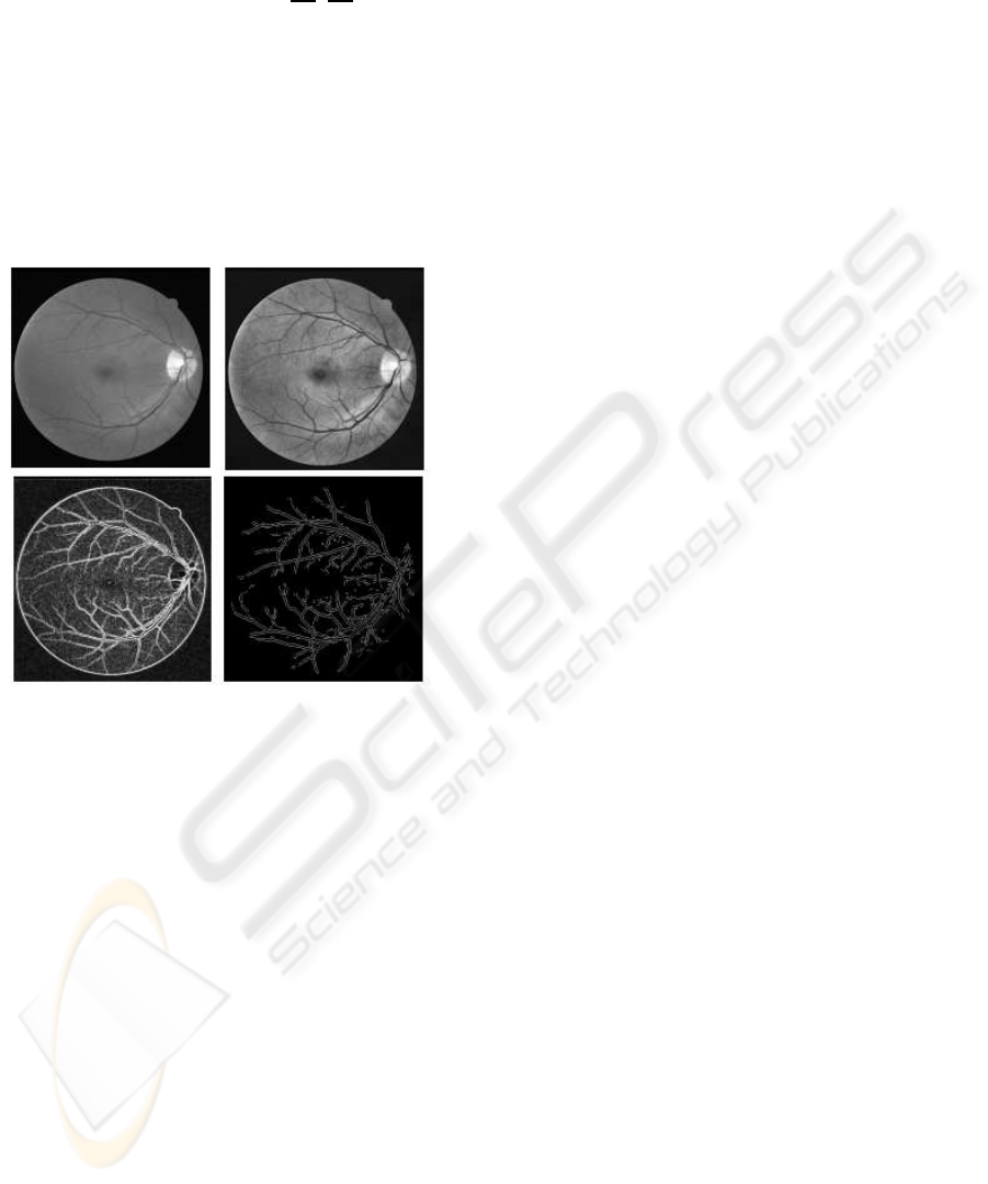
4.4 Experimental Results
Using the DRIVE database (DRIVE-database, 2004)
we applied our method on five images for vessel seg-
mentation. For performance evaluation, we detected
the vessel centerline in our output segmented im-
ages and hand-labeled ground truth segmented (GT)
images applying the morphological thinning opera-
tion (Figure 5). We achieved an overall 84.37%
sensitivity (TP/(TP + FN)) and 99.61% specificity
(TN/(TN + FP)) where TP, TN, FP and FN are true
BIOSIGNALS 2008 - International Conference on Bio-inspired Systems and Signal Processing
182
positive, true negative, false positive and false nega-
tive respectively. Hoover et al. (Hoover et al., 2000)
method on the same five segmented images provided
in 68.23% sensitivity and 98.06% specificity. Clearly,
our method produces superior results.
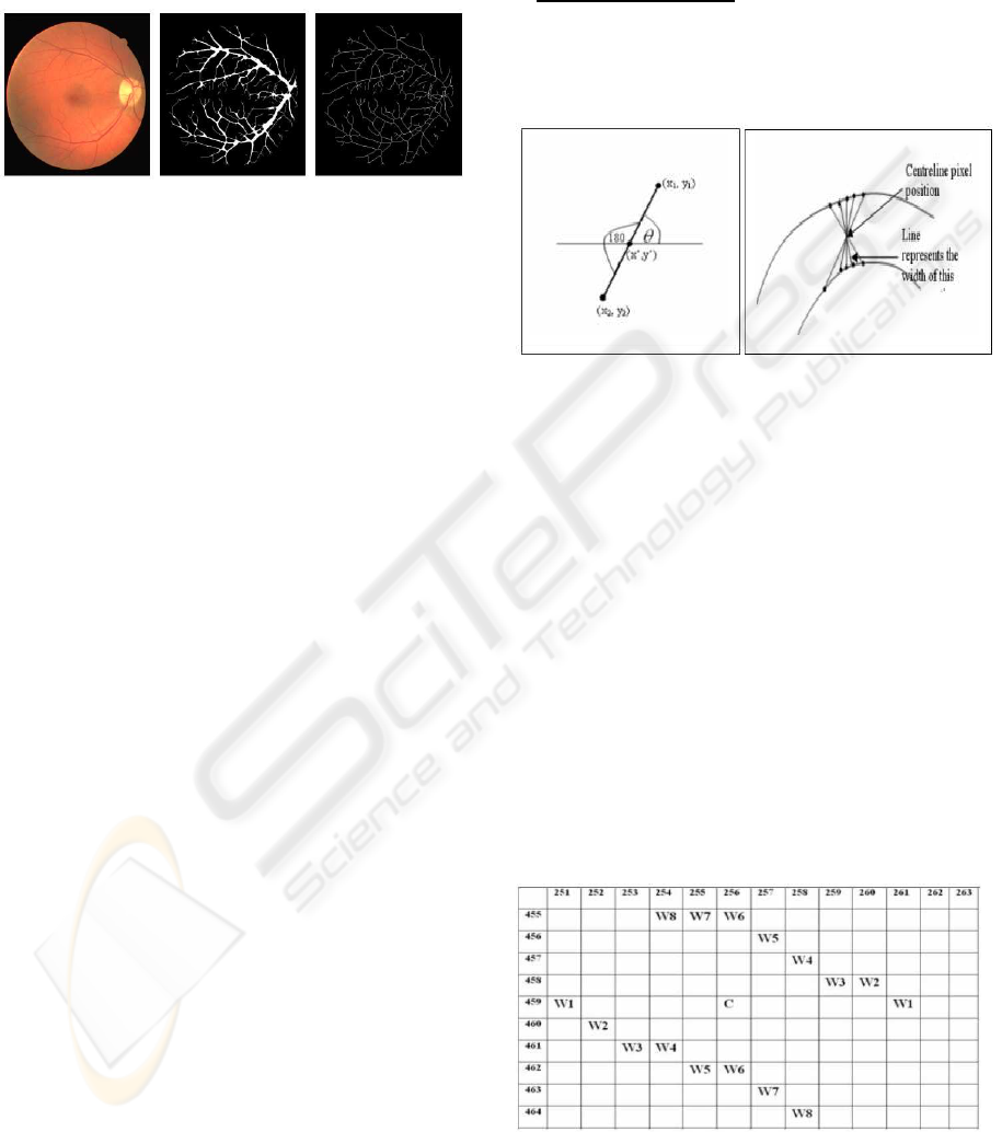
Figure 5: Original RGB image, vessel segmented image,
and its centreline image (from left to right).
5 VESSEL WIDTH
MEASUREMENT
After obtaining the vessels edge image and centre-
line image, we mapped these images to find the vessel
width for a particular vessel centreline pixel position.
To do this we first pick a pixel from the vessel cen-
treline image, then we apply a mask considering this
centreline pixel as its centre. The purpose of this mask
is to find the potential edge pixels (which may fall in
width or cross section of the vessels) in any side of
that centreline pixel position. Therefore, we will ap-
ply the mask to the edge image only. For searching all
the pixel positions inside the mask, we calculate the
pixel position by shifting by one up to the size of the
mask and rotating each position from 0 to 180 degrees
at the same time. For increasing the rotation angle we
use the step size (depending on the size of the mask)
less then 180/(mask length). Therefore, we can access
every cell in the mask using this angle.
For each obtained position we search the edge im-
age gray scale value to check whether it is an edge
pixel or not. Once we find an edge pixel we then find
it’s mirror by shifting the angle of 180 degree and in-
creasing the distance from one to the maximum size
of the mask (Figure 6). In this way we produce a ro-
tational invariant mask and pick all the potential pixel
pairs to find the width or diameter of that cross sec-
tional area.
x1 = x
′
+ r∗ cosθ
y1 = y
′
+ r∗ sinθ
(12)
where (x
′
,y
′
) is the vessel centreline pixel position,
r=1,2,..(mask size)/2 and θ = 0, ..,180
o
. For any pixel
position, if the gray scale value in the edge image
is 255 (white or edge pixel) then we find the pixel
(x2,y2) in the opposite edge (mirror of this pixel) con-
sidering θ = (θ+ 180) and varying r.
After applying this operation we obtain the pairs
of pixels which are on the opposite edges (at line
end points) giving imaginary lines passing through
the centerline pixels (Figure 6). From these pix-
els pairs we find the minimum Euclidian distance
p
(x
1
− x
2
)
2
+ (y
1
− y
2
)
2
, the width of that crosssec-
tion. In this way, we can measure the width for all
vessels including the vessels’ with one pixel wide (for
which we have the edge and the centreline itself).
Figure 6: Finding the mirror of an edge pixel(left) and width
or minimum distance from potential pairs of pixels (right).
6 EXPERIMENTAL RESULTS
AND DISCUSSION
We used the centreline images and edge images for
measuring the width of the blood vessels. We mea-
sure the accuracy qualitatively by comparing with the
width measured by plotting the centreline pixel and
its surround edge pixels. We considered ten different
vessel cross-sections of these images and observed
that our method is working very accurately. Figure
7 portrays the Grid for a cross-section of a blood ves-
sel where c is the centreline pixel and w1 to w8 are
potential width end points. Figure 8 depicts the de-
tected width for some cross-sectional points indicat-
ing in white lines (enlarged).
Figure 7: Grid showing the potential width edge pairs for a
cross-section with centreline pixel C.
For quantitative evaluation we considered ten
images (each 3072×2048 which captured with the
AN EFFICIENT METHOD FOR VESSEL WIDTH MEASUREMENT ON COLOR RETINAL IMAGES
183
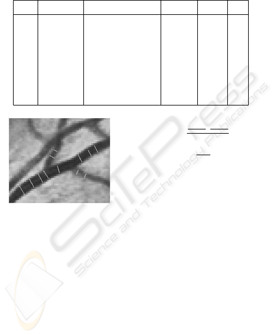
Table 1: Measuring the accuracy of the automatic width measurement.
Cross- Centreline pixel Detected width end points Auto. width Accuracy Error
section X
c
Y
c
X
1
Y
1
X
2
Y
2
(A) (%) (%)
1 2055 629 2068 632 2046 628 22.361 99.14 0.86
2 1859 519 1871 519 1850 520 21.024 97.50 2.50
3 2259 815 2259 811 2259 824 13 99.46 0.54
4 2350 1077 2350 1070 2350 1084 14 87.61 12.39
5 2233 1317 2239 1314 2239 1322 11.314 93.49 6.51
6 2180 1435 2189 1431 2172 1440 19.235 95.39 4.61
7 2045 1451 2055 1452 2042 1452 13 85.55 14.45
8 1683 1500 1691 1509 1680 1496 17.029 87.52 12.48
9 1579 617 608 1593 630 1573 23.409 98.48 1.52
10 1434 855 853 1436 859 1432 7.211 85.48 14.52
11 1443 1000 999 1446 1004 1440 7.81025 91.23 8.77
12 1618 1331 1335 1623 1330 1617 7.81025 89.54 10.46
13 1475 1164 1169 1479 1162 1474 8.6023 83.20 16.80
Figure 8: Measured vessel width showing by the white lines
in an image portion.
Canon D-60 digital fundus camera) with manually
measured width on different cross-sections from
Eye and Ear Hospital, Victoria, Australia. For each
cross-section, we received the graded width by
five different experts who are trained retinal vessel
graders of that institution. For manual grading a
computer program was used where the graders could
zoom in and out at will, moving around the image
and selecting various parts. We applied our technique
on these images to produce the edge image and vessel
centreline image. We considered these images and
randomly picked ninety-six cross-sections of vessels
varying width from one to twenty-seven pixels. We
measured the width for each cross-section by our
automatic width measurement technique (we call it
automatic width, A) and considered the five manually
measured width (we call it manual width) by experts.
We calculated the average of the manual width
(µ), the standard deviation on manual widths (σ
m
)
and considered the following formula to find the error,
E =
(µ−σ
m
)−A
(µ−σ
m
)
+
(µ+σ
m
)−A
(µ+σ
m
)
2
=
1−
µ×A
µ
2
−σ
2
m
(13)
In equation (13), we considered (µ ± σ
m
) to normal-
ize it. This formula is a good measure as the error
rate will be less if it is within the interval one stan-
dard deviation. With this formula, we calculated the
error and accuracy in all ninety-six cross-section and
achieve an average of 95.8% accuracy (maximum ac-
curacy is 99.58% and minimum accuracy is 83.20%)
in the detection of vessel width. We found the max-
imum error is 16.80% which is 2.04 pixel and the
minimum error is 0.698% which is 0.139 pixel. Ta-
ble 1 and 2 depict the manual and automatic width
measurement accuracy on different cross-sections in
an image. We compared our technique with (Lowell
et al., 2004) which achieved the maximum accuracy
of 99% (did not mention the average accuracy for all
cross-sections) with minimum pixel error of 0.34. Us-
ing the same formula, |(µ−A)/µ|), we achieved 100%
accuracy. Clearly, our technique is performing better.
7 CONCLUSIONS AND FUTURE
WORK
In this paper we proposed a new and efficient tech-
nique for blood vessels width measurement. This ap-
proach is a robust estimator of vessel width in the
presence of low contrast and noise. The results ob-
tained are promising and the detected width can be
used to measure different parameters (nicking, nar-
BIOSIGNALS 2008 - International Conference on Bio-inspired Systems and Signal Processing
184
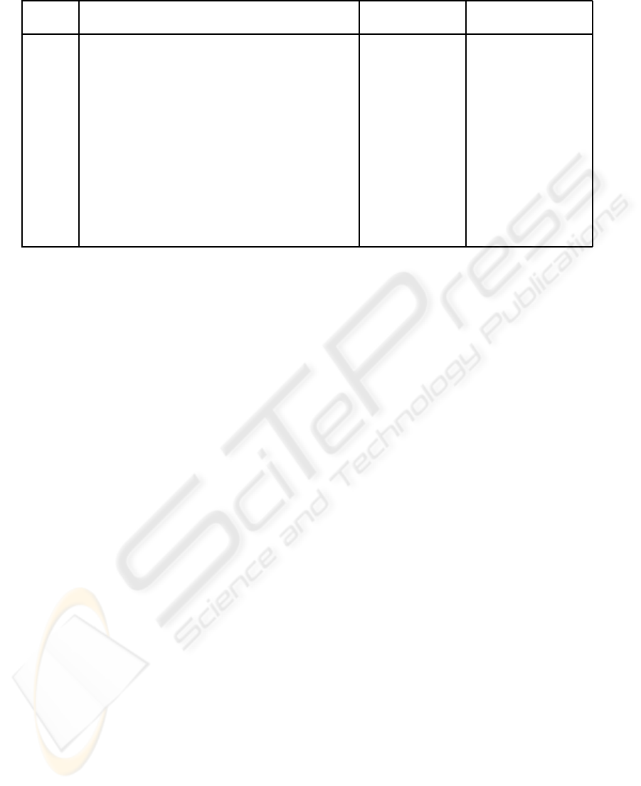
Table 2: Manually measured widths for an image cross-sections.
Cross- Manually measured width (in Micron) Mean width (µ) Standard Deviation
section One Two Three Four Five (in pixel) (σ
m
)
1 112.42 117.53 107.31 117.53 112.42 22.2 0.8366
2 107.31 112.42 107.31 117.53 107.31 21.6 0.8944
3 66.43 76.65 61.32 71.54 61.32 13.2 1.3088
4 61.32 71.54 61.32 71.54 56.21 12.6 1.3416
5 56.21 66.43 56.21 66.43 66.43 12.2 1.0954
6 107.31 107.31 102.2 102.2 97.09 20.2 0.8366
7 56.21 66.43 45.99 61.32 66.43 11.6 1.6733
8 86.87 107.31 102.2 107.31 97.09 19.6 1.6733
9 132.86 127.75 112.42 132.86 107.31 24 2.3452
10 45.99 51.1 35.77 56.21 35.77 8.8 1.7889
11 40.88 56.21 35.77 45.99 45.99 8.8 1.4832
12 35.77 51.1 45.99 56.21 40.88 9 1.5811
13 35.77 45.99 35.77 45.99 30.66 7.6 1.3416
rowing, branching coefficients, etc.) for diagnosing
various diseases. Currently, we are working on the
blood vessels’ bifurcation and cross-over detection
where the measured width is contributing as an im-
portant information for perceptual grouping process.
ACKNOWLEDGEMENTS
We would like to thank David Griffiths (Research As-
sistant, The University of Melbourne and Eye and Ear
Hospital, Melbourne, Australia) for providing us with
the manually measured width images and data.
REFERENCES
Bezdek, J. (1981). Pattern recognition with fuzzy objective
function algorithms. Plenum Press, USA.
Bhuiyan, A., Nath, B., and Chua, J. (2007a). An adaptive
region growing segmentation for blood vessel detec-
tion from retinal images. Second International Con-
ference on Computer Vision Theory and Applications,
pages 404–409.
Bhuiyan, A., Nath, B., Chua, J., and Kotagiri, R. (2007b).
Blood vessel segmentation from color retinal images
using unsupervised classification. In the proceedings
of the IEEE International Conference of Image Pro-
cessing.
Brinchman-hansan, O. and Heier, H. (1986). Theoritical re-
lations between light streak characterstics and optical
properties of retinal vessels. Acta Ophthalmologica,
179(33).
DRIVE-database (2004). http://www.isi.uu.nl/research/
databases/drive/, image sciences institute, university
medical center utrecht, the netherlands.
Gao, X., Bharath, A., Stanton, A., Hughes, A., Chapman,
N., and Thom, S. (2001). Measurement of vessel
diameters on retinal images for cardiovascular stud-
ies. Proceedings of Medical Image Understanding
and Analysis, pages 1–4.
Geusebroek, J., Boomgaard, R. V. D., Smeulders, A. W. M.,
and Geerts, H. (2001). Color invariance. IEEE Trans-
actions on Pattern Analysis and Machine Intelligence,
23(2):1338–1350.
Gonzalez, R. C., Woods, R. E., and Eddins, S. L. (2004).
Digital image processing using matlab. Prentice Hall.
Hoover, A., Kouznetsova, V., and Goldbaum, M. (2000).
Locating blood vessels in retinal images by piece-wise
threshold probing of a matched filter response. IEEE
Transactions on Medical Imaging, 19(3):203–210.
Kruizinga, P. and Petkov, N. (1999). Nonlinear operator for
oriented texture. IEEE Transactions on Image Pro-
cessing, 8(10):1395–1407.
Lowell, J., Hunter, A., Steel, D., Basu, A., Ryder, R.,
and Kennedy, R. L. (2004). Measurement of reti-
nal vessel widths from fundus images based on 2-d
modeling. IEEE Transactions on Medical Imaging,
23(10):1196–1204.
Wu, D., Zhang, M., and Liu, J. (2006). On the adaptive de-
tetcion of blood vessels in retinal images. IEEE Trans-
actions on Biomedical Engineering, 53(2):341–343.
Wyszecki, G. W. and Stiles, S. W. (1982). Color science:
Concepts and methods, quantitative data and formu-
las. New York, Wiley.
Zhou, L., Rzeszotarsk, M. S., Singerman, L. J., and Chokr-
eff, J. M. (1994). The detection and quantification of
retinopathy using digital angiograms. IEEE Transac-
tions on Medical Imaging, 13.
AN EFFICIENT METHOD FOR VESSEL WIDTH MEASUREMENT ON COLOR RETINAL IMAGES
185
