MODEL ORDER ESTIMATION FOR INDEPENDENT COMPONENT
ANALYSIS OF EPOCHED EEG SIGNALS
Peter Mondrup Rasmussen, Morten Mørup, Lars Kai Hansen
Informatics and Mathematical Modelling, Technical University of Denmark
Richard Pedersens Plads, bld. 321, DK-2800 Kgs. Lyngby, Denmark
Sidse M. Arnfred
Cognitive Research Unit, Department of Psychiatry, University Hospital of Copenhagen, Hvidovre
Brøndbyøstervej 160, DK-2605 Brøndby, Denmark
Keywords:
EEG, Event related potentials, Independent component analysis (ICA), Molgedey Schuster, TDSEP, Model
selection, Cross validation.
Abstract:
In analysis of multi-channel event related EEG signals indepedent component analysis (ICA) has become
a widely used tool to attempt to separate the data into neural activity, physiological and non-physiological
artifacts. High density elctrode systems offer an opportunity to estimate a corresponding large number of
independent components (ICs). However, too large a number of ICs leads to overfitting of the ICA model,
which can have a major impact on the model validity. Consequently, finding the optimal number of compo-
nents in the ICA model is an important problem. In this paper we present a method for model order selection,
based on a probabilistic framework. The proposed method is a modification of the Molgedey Schuster (MS)
algorithm to epoched, i.e. event related data. Thus, the contribution of the present paper can be summarized
as follows: 1) We advocate MS as a low complexity ICA alternative for EEG. 2) We define an epoch based
likelihood function for estimation of a principled unbiased ’test error’. 3) Based on the unbiased test error
measure we perform model order selection for ICA of EEG. Applied to a 64 channel EEG data set we were
able to determine an optimum order of the ICA model and to extract 22 ICs related to the neurophysiological
stimulus responses as well as ICs related to physiological- and non-physiological noise. Furthermore, highly
relevant high frequency response information was captured by the ICA model.
1 INTRODUCTION
The electroencephalogram (EEG) is a recording of
electrophysiological brain activity and the major ben-
efit of EEG relative to other brain imaging modali-
ties is a high temporal resolution. The basic elec-
trophysiology of the EEG signal implies that it may
be modelled as a linear mixture of multiple sources
of neural activity, non-brain physiological artifacts
such as eye blinks, eye movements, and muscle activ-
ity, and non-physiological artifacts such as line noise,
and electrode movement (Onton et al., 2006; Hesse
and James, 2004). By electrical conductance these
source signals instantaneously project to the scalp
electrodes used for acquisition (Onton et al., 2006).
Assuming linear addition of these relatively indepen-
dent source signals at the scalp electrodes motivates
the use of instantaneous independent componentanal-
ysis (ICA) as a technique for extracting a set of under-
lying sources from the recorded EEG signals (James
and Hesse, 2005; Makeig et al., 2002; Hyvarinen and
Oja, 2000). The EEGLAB software is widely used for
decomposing EEG using ICA (Delorme and Makeig,
2004). More accurate modeling of the signal com-
ponent(s) including residual delayed correlations can
be achieved using so-called convolutive ICA in a sub-
space of components extracted by the initial instanta-
neous ICA (Dyrholm et al., 2007).
Epochs extracted from an EEG experiment are de-
scribed by the data matrix X ∈ R
M×N
, where M is
the number of electrode channels and N is the number
of sampling time points. In the following N is the to-
tal time consisting of a certain number of epochs, i.e.,
individual experiment. The epochs may be separated
by variable time intervals according to the specific ex-
perimental design. It is a specific point in the follow-
ing, where we are going to invoke temporal correla-
tion based models, that we do not compute temporal
3
Mondrup Rasmussen P., Mørup M., Kai Hansen L. and M. Arnfred S. (2008).
MODEL ORDER ESTIMATION FOR INDEPENDENT COMPONENT ANALYSIS OF EPOCHED EEG SIGNALS.
In Proceedings of the First International Conference on Bio-inspired Systems and Signal Processing, pages 3-10
DOI: 10.5220/0001059500030010
Copyright
c
 SciTePress

correlations across epoch boundaries.
In general the ICA model can be written as
X = AS X
n,t
=
K
X
k=1
A
n,k
S
k,t
, (1)
where X
n,t
is the signal at the n
′
th sensor at t
′
th time
point and K is the number of sources or independent
components (ICs). A ∈ R
M×K
is denoted the mix-
ing matrix and S ∈ R
K×N
the source matrix. In this
model the sources as well as the mixing coefficients
are unknown. The random signal X is observed, and
from this A and S are estimated. It is impossible to
determine the variance (energy) of the sources, since
any scalar multiplier in one of the sources could be
cancelled by dividing the corresponding column in A
with the same multiplier. Therefore, the sources are
often assumed to have unit variance, which can be
achieved by normalizing the source signals and mul-
tiply the corresponding column of the mixing matrix.
Specifically, there is a sign ambiguity, if we change
the sign of a source signal and change the sign of
the corresponding column in the mixing matrix, the
same reconstructed signal is obtained by multiplica-
tion. Finally, the ordering of components is arbitrary.
We may order independent component according to
variance of their contribution to the reconstructed sig-
nal.
The recovery of the mixing matrix and the sources
is not possible from the covariance matrix alone,
hence, by principal component analysis (PCA). Addi-
tional information is needed. ICA is often based on a
non-Gaussianity assumption of the sources (Bell and
Sejnowski, 1995) or by assumed differences in source
auto-correlation (Molgedey and Schuster, 1994).
The number of EEG channels M may be differ-
ent from the number of sources K, thus it is relevant
to estimate K. Estimation of the correct number of
sources can have a major impact on the validity of
the ICA solution and prevents overfitting (James and
Hesse, 2005). One approach to prevent overfitting is
based on pre-processing by PCA, where the number
of sources is determined by the number of dominant
eigenvalues which account for a high proportion of
the total variance in the data set. However this proce-
dure has been criticized for sensitivity to noise (James
and Hesse, 2005). Another approach is based on step-
wise extraction of sources until a specified accuracy
is achieved (James and Hesse, 2005). However this
method is highly dependent on the choice of the ac-
curacy level. In this paper we present a method for
model order selection, based on a probabilistic frame-
work. This approach was earlier proposed in a multi-
media contexts (Kolenda et al., 2001). However, the
approach requires large amount of memory for long
signals and is inapplicable to EEG signals that are
epoched due to temporal discontinuities where epochs
are merged. Here we present a method that is cus-
tomized to epoched data with the additional benefit
of reducing the memory requirement. In our method
PCA leads to a number of model hypotheses, of which
an ICA model is estimated using a modified version
of the Molgedey Schuster (MS) algorithm (Molgedey
and Schuster, 1994). The MS algorithm is chosen be-
cause it is based on source autocorrelation, which is
very relevant to EEG, and because of its relative low
computational complexity. We take further advantage
of the epoched nature of the signals, and split the data
set into a training- and a test set. Model selection, i.e.,
estimating K, is then based on evaluating the likeli-
hood of each model hypothesis using the test set in
order to ensure generalization.
The paper is organized as follows. First we give a
description of our method and we compare by sim-
ulation study the modified MS algorithm with the
currently used ICA methods for EEG TDSEP (Ziehe
et al., 2000) and infomax ICA (Bell and Sejnowski,
1995). We then test our model selection scheme
within the simulated data and apply our method on
real event related EEG data from an experiment in-
volving visual stimulus.
2 METHODS
In the following, a description of PCA and the MS
algorithm will be given. This is followed by a de-
scription of the probabilistic modelling. Finally the
procedures for model order selection is presented.
2.1 PCA
Using PCA it is possible to reduce the dimension-
ality of the ICA model. In EEG M ≪ N which
leads to the singular value decomposition (SVD) X =
UDV
T
, where U ∈ R
M×M
, D ∈ R
M×N
, and
V ∈ R
N×N
. By selecting the first K eigenvectors
in U as a new basis, the signal space S is reduced to
K dimensions. ICA is performed in S, where A is the
ICA basis projected onto the PCA subspace. The mix-
ing matrix in the original vector space and the source
signals are then given by
˜
A = U A (2)
S = A
−1
DV
T
. (3)
The noise space E is spanned by the remaining M −K
eigenvectors.
BIOSIGNALS 2008 - International Conference on Bio-inspired Systems and Signal Processing
4

2.2 Molgedey Schuster Separation
The Molgedey Schuster approach is based on the
assumption that the autocorrelation functions of the
independent sources are non-vanishing, and can be
used if the source signals have different autocorrela-
tion functions (Molgedey and Schuster, 1994; Hansen
et al., 2000; Hansen et al., 2001). Time shifted data
matrices X
τ
and S
τ
are defined followed by the defi-
nition of the cross-correlation function matrix for the
mixture signals
C(τ) ≡
1
N
e
X
τ
X
T
, (4)
where C ∈ R
M×M
and N
e
is the epoch length.
For τ = 0 the usual cross-correlation matrix is ob-
tained. Due to the epoched nature of the signals C(τ )
is estimated within each epoch and averaged, since
the cross-correlation is not valid over epoch bound-
aries. Now we define the quotient matrix Q(τ) ≡
C(τ)C(0)
−1
which is rewritten, using the relation
X = AS, as
Q(τ) = C(τ)C(0)
−1
=
1
N
e
X
τ
X
T
(
1
N
e
XX
T
)
−1
= (AS
τ
)(AS)
T
((AS)(AS)
T
)
−1
= AS
τ
S
T
A
T
A
−T
(SS
T
)
−1
A
−1
= AD(τ )D(0)
−1
A
−1
, (5)
where D(τ) ≡
1
N
e
S
τ
S
T
in the limit N
e
→ ∞ is the
diagonal source cross-correlation matrix at lag τ . It
is now seen, that the eigenvalue decomposition of the
quotient matrix
QΦ = ΦΛ (6)
leads to A = Φ and Λ = C(τ)C(0)
−1
. τ is estimated
as described in (Kolenda et al., 2001).
2.3 Probabilistic Modeling
The ICA model is defined in terms of the model pa-
rameters i.e. the mixing matrix A. Using Bayes
theorem the probability of specific model parameters
given the observed data P (A|X) can be written as
P (A|X) =
P (X|A)P (A)
P (X)
, (7)
where P (X|A) is the likelihood function, and P (A)
is the prior probability of a specific model. This like-
lihood function is rewritten as
P (X|A) =
Z
P (X, S|A)dS
=
Z
P (X|S, A)P (S)dS
=
Z
δ(X − AS)P (S)dS (8)
Evaluating the integral in (8) gives
P (X|A) = P (A
−1
X)
1
||A||
, (9)
where ||A|| is the absolute determinant of A.
In order to write the likelihood function we need
the likelihood for the reduced signal space S as well
as for the noise space E. Since the sources are sta-
tistically independent we have P (S) =
Q
K
i=1
P (s
i
),
where s
i
denotes the i’th source. If the sources are
assumed stationary, independent, have zero mean,
possess time-autocorrelation and are Gaussian dis-
tributed, then the source distribution is given by
(Hansen et al., 2001; Hansen et al., 2000)
P (S) =
K
Y
i=1
1
p
|2πΣ
s
i
|
exp

−
1
2
s
T
i
Σ
−1
s
i
s
i

, (10)
where Σ
s
i
= E[s
i
s
T
i
] = T oepli t z([γ
s
i
(0), ...
, γ
s
i
(N
e
− 1)]) and γ
s
i
are the source autocorrelation
function values. The autocorrelation function values
are estimated in each epoch and averaged. This esti-
mate of the source distribution leads to a formulation
of the likelihood for the signal space as
P (S|A) =
K
Y
i=1
1
p
|2πΣ
s
i
|

1
||A||

N
e
× exp

−
1
2
s
−1
i
Σ
T
s
i
s
i
)

. (11)
The noise space E is assumed to be isotropic with
noise variance σ
2
E
= (M −K)
−1
P
M
i=K+1
D
2
ii
. It can
be shown (Kolenda et al., 2001; Minka, 2001) that
P (E|σ
2
E
) =

2πσ
2
E

−
N
e
(M−K)
2
× exp

−
N
e
(M − K)
2

. (12)
The signal and noise space are assumed independent
which leads to the likelihood function
P (X|A) = P (S|A)P (E|σ
2
E
). (13)
2.4 Model Order Selection
PCA reduction of dimensionality leads to a set of M
model hypotheses. Since the data set consists of a
MODEL ORDER ESTIMATION FOR INDEPENDENT COMPONENT ANALYSIS OF EPOCHED EEG SIGNALS
5

large number of epoch e.g. 105, we have the opportu-
nity to split the data set into a training set D
tr ain
and
a test set D
test
. Using D
tr ain
the model parameters A
and Σ
s
i
in (11) are estimated. The negative logarithm
of the likelihood function (13) is then evaluated using
D
test
, where (11) is rewritten as
− lo g (P (S|A)) = N
e
log(||A||)
+
1
2
N
e
+ K log(2π) +
1
2
K
X
i=1
log(


Σ
s
i,train


)
+
1
2
K
X
i=1
T r(Σ
s
i,test
Σ
−1
s
i,train
), (14)
where N
e
is the number of samples in each epoch ,
||A|| is the absolute determinant of A estimated from
D
tr ain
, K is the dimension of D and Σ
s
i,train
and
Σ
s
i,test
are estimated from D
tr ain
and D
test
respec-
tively. By observing (13) model order selection is per-
formed by identifying the model order having mini-
mal generalization error.
3 EXPERIMENTAL EVALUATION
Simulation experiments was conducted to investigate
the performance of the MS algorithm and the test set
procedure for model order selection. The data sets are
constructed from three sources s
1
, s
2
, and s
3
which
show bursts at frequencies of 14, 19, and 11 Hz re-
spectively. The simulated source signal matrix S con-
sist of 80 epochs of bursts with random intra epoch in-
terval. A 50 Hz noise source s
4
is included after gen-
eration of the 80 epochs. Electrode signals are created
by mixing the simulated source signals with a speci-
fied mixing matrix A, and Gaussian noise E is added
to the electrode signals leading to a specic signal-to-
noise ratio (SNR) (a description of noise generation
is found in Appendix). Epochs are extracted from the
mixed signals using EEGLAB (Delorme and Makeig,
2004).
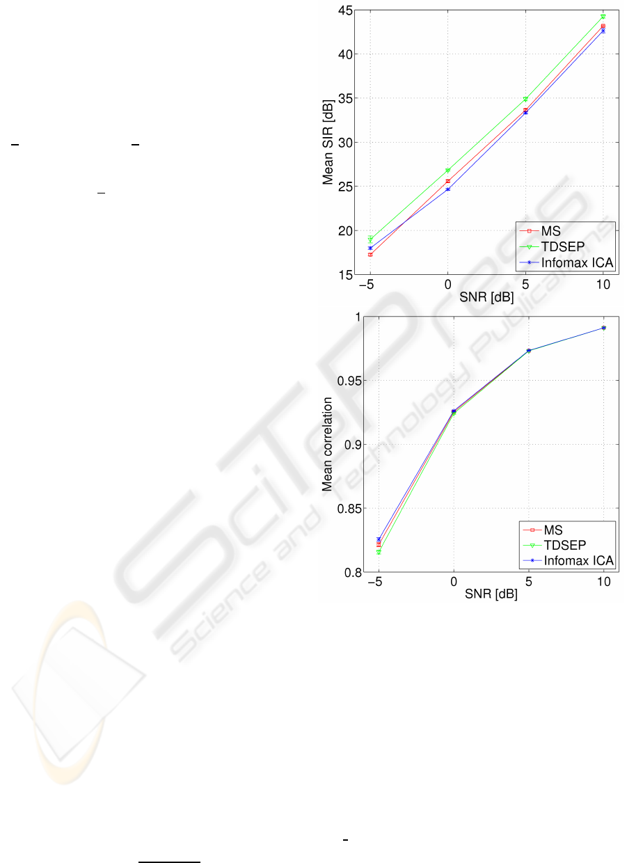
3.1 Algorithm Performance Results
By PCA the dimensionality of the simulation was
reduced to 4 dimensions, and the ICA model esti-
mated by TDSEP, the infomax ICA implementation
of EEGLAB, and our modified MS algorithm. To
evaluate the separation performance of our algorithm,
we use the correlation between original- and esti-
mates sources as well as the source-to-interferencera-
tio (SIR) (Fevotte et al., 2005; Vincent et al., 2006)
measure
SIR = 10 log
10
||s
target
||
2
||e
interf
||
2
, (15)
Figure 1: Simulation experiment. Results for source sep-
aration for TDSEP (Applied with default timelags 0,1),
EEGLAB’s implementation of infomax ICA, and our epoch
modified MS algorithm. The simulation data is constructed
from four signal sources mixed out in 32 channels, Gaussian
noise is added. Dimensional reduction to four dimensions
by PCA. Experiment repeated 10 times, error bars indicate
three standard deviations of the mean. Top: Performance
of source estimation measured in terms of mean SIR. Bot-
tom: Performance measured in terms of mean correlation
between true sources and estimates.
where s
target
represents the target source or true
source and e
interf
represents interferences of un-
wanted sources. The SIR was calculated using the
BSS EVAL toolbox (Fevotte et al., 2005), where the
performance measure is computed for each estimated
source ˆs
i
by comparing it to the true source s
i
and
BIOSIGNALS 2008 - International Conference on Bio-inspired Systems and Signal Processing
6

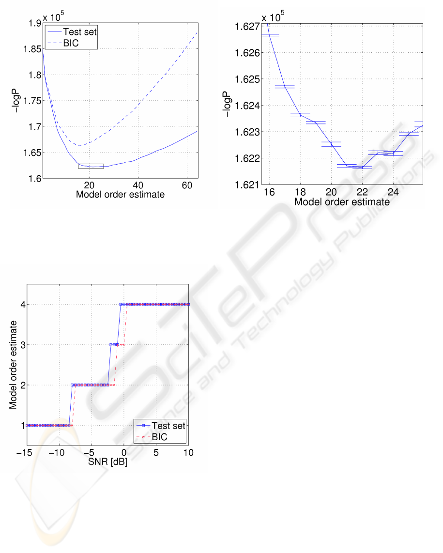
Figure 3: Left: Negative log likelihood for each of the 64 model hypotheses. Test set curve is averaged over 10 experiments,
and minimum is found at 22 dimensions, suggesting an ICA model with 22 ICs. BIC is more conservative and estimates
16 ICs. Right: Zoom of the minimum region in the test set curve indicated by the box on left plot. Errorbars indicate three
standard deviations of the mean.
Figure 2: Simulation experiment. Results for model or-
der selection for the test set procedure and for BIC estima-
tion. The simulation is constructed from four signal sources
mixed out in 32 channels, and Gaussian noise is added. BIC
underestimates the number of sources at 0 dB whereas the
test set procedure remains stable until -1 dB.
other unwanted sources (s
j
)
j6=i
. In general SIR lev-
els below 8-10 dB indicate failure in separation (Bos-
colo et al., 2004). Figure 1 shows that source esti-
mates achieved with the modified MS algorithm are
comparable with results from the alternative ICA al-
gorithms. The MS algorithms has the advantages that
it is fast compared to infomax ICA and TDSEP. Fur-
thermore, there exists a heuristic for estimation of the
time lag parameter τ.
3.2 Model Estimation
Model order selection is performed using the test
set likelihood function (13) as evaluated using 10-
fold cross-validation. Figure 2 shows model or-
der estimates for a wide range of SNR. Here the
proposed cross-validation procedure is compared to
the Bayesian Information Criterion (BIC) (MacKay,
1992). The experiment indicates, that the cross-
validation procedure is more robust than BIC estima-
tion but it also has a tendency to underestimate the
number of sources at low SNR.
4 APPLICATION ON EEG DATA
SET
Our model selection procedure was applied on a data
set from a visual stimulation experiment with exper-
imental details described in (Mørup et al., 2006) and
paradigm described in (Herrmann et al., 2004). EEG
was recorded with 64 scalp electrodes arranged ac-
cording the the International 10-10 system, sampling
frequency 2048 Hz, band pass filter 0.1-760 Hz. Data
MODEL ORDER ESTIMATION FOR INDEPENDENT COMPONENT ANALYSIS OF EPOCHED EEG SIGNALS
7

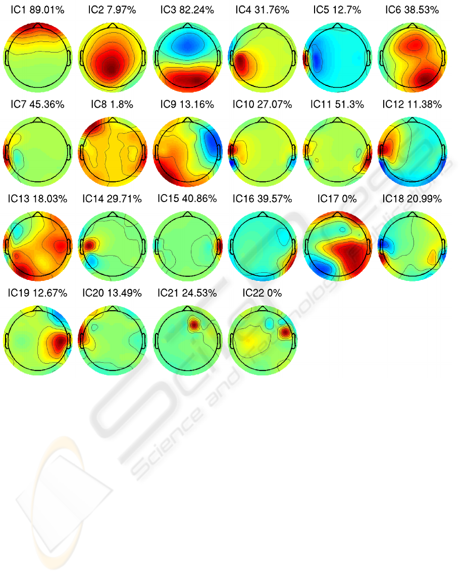
Figure 4: Interpolated scalp maps individually scaled to maximum absolute values. Dimensionality of the data from 64 scalp
electrodes reduced to 22 by PCA. ICs estimated by MS algorithm, and components are sorted according to variance. The
percentage at each IC indicates how much variation is explained by the respective IC of the average ERP at the electrode,
where the respective IC project the strongest, calculated as (||X
k
||
2
F
− ||X
k
− P
k
||
2
F
)/||X
k
||
2
F
, where X
k
is the ERP at
electrode k and P
k
is the projection ERP of the respective IC onto electrode k. Estimated ICs represents different types of
sources, for example, IC1 reflects eye artifacts, IC2, IC3, IC4, IC6 reflect brain sources and IC21, IC22 reflect electrode noise.
was high pass filtered at 3 Hz in EEGLAB, and line
noise removed using a maximum likelihood 50 Hz
filter. The data were referenced to digitally linked
earlobes, down sampled to 256 Hz and cut into 105
epochs (-500 to 1500 ms).
PCA leads to a set of 64 model hypotheses. For
each hypothesis the negative logarithm of the likeli-
hood function (13) was evaluated using 10-fold cross-
validation. The experiment was repeated 10 times
with different splits of training- and test sets. Figure
3 shows model order estimation by the test set proce-
dure and BIC estimation.
According to model order estimation the dimen-
sionality of the data set was reduced to 22 by PCA.
ICs were estimated by the MS algorithm and sorted
according to variance. Figure 4 shows all IC scalp
maps. To categorize components each scalp map and
averaged event related potentials (ERPs) were exam-
ined, where for example IC2, IC3, IC4 and IC6 reflect
brain sources, IC1 reflects physiological eye artifacts,
and IC21 and IC22 reflect electrode noise.
Further analysis of IC3 is performed by creating
ERP images (Delorme and Makeig, 2004) as shown
in Figure 5 top, from the PO4 electrode signal and
IC3 projected onto electrode PO4. Generally the elec-
trode signal has a larger amplitude than the projec-
tion of IC3, however, the major dynamics of the ERP
seems to be captured by IC3. Another common analy-
BIOSIGNALS 2008 - International Conference on Bio-inspired Systems and Signal Processing
8

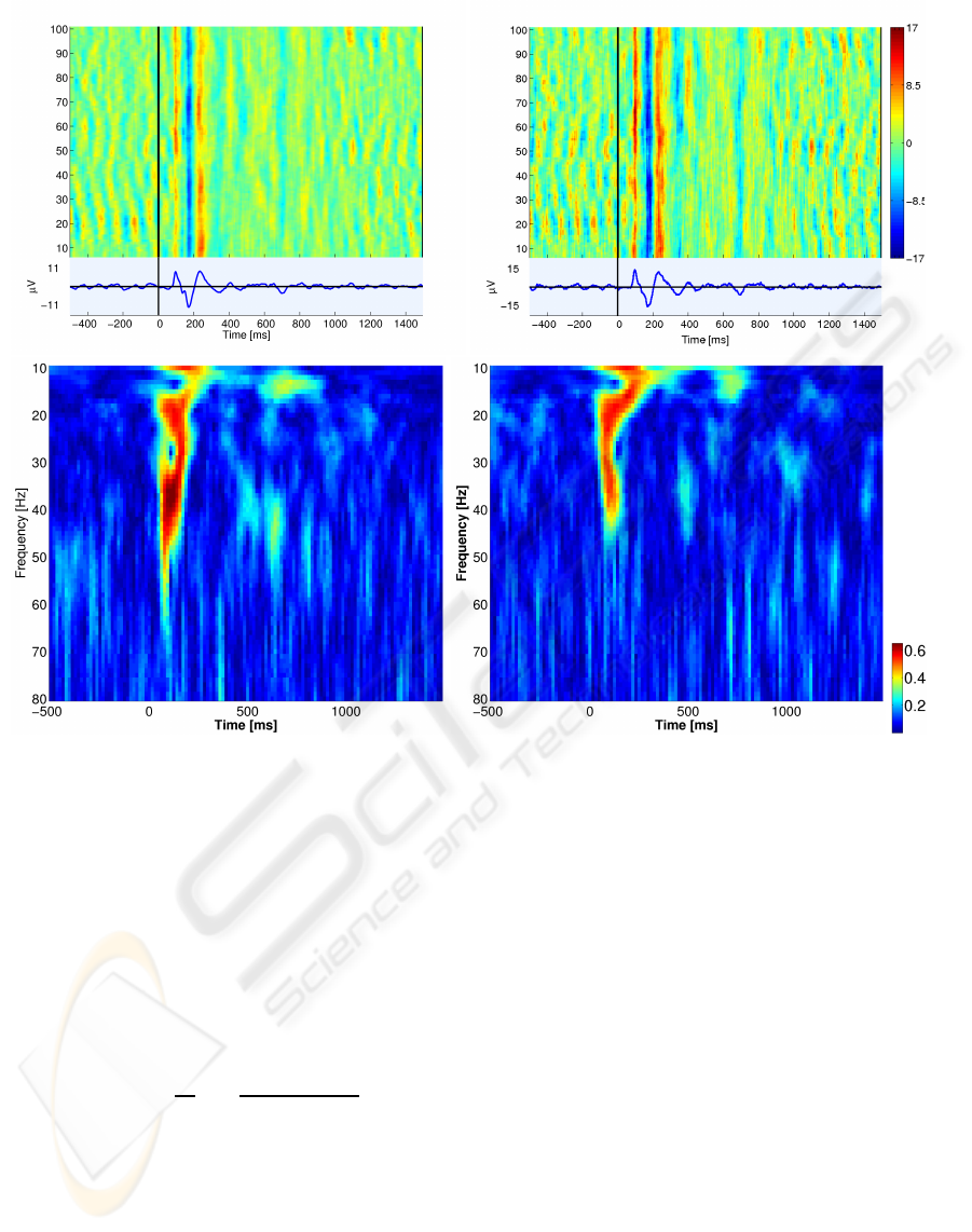
Figure 5: Top panel; ERP images, scaled to same color scale, epochs sorted by epoch number. Left; Image of IC3 projected
onto electrode PO4. Right; Electrode signal at PO4. The electrode signal has a larger amplitude than the projection of IC3,
however, the major dynamics of the ERP seems to be captured in IC3. Bottom panel; Time-frequency plots of the ITPC scaled
to same color scale. Left; IC3 projected onto electrode PO4. Right; Electrode signal at PO4. IC3 reveals prominent evoked
activity in the gamma band around 40 Hz compared to the raw electrode signal.
sis tool is time-frequency analysis of ERPs (Delorme
and Makeig, 2004; Mørup et al., 2007), where differ-
ent time-frequency measures exist. By ERPWAVE-
LAB (Mørup et al., 2007) we wavelet transformed the
data using the complex Morlet wavelet and calculated
the inter-trial phase coherence (ITPC)
IT P C(c, f, t) =
1
N
N
X
n=1
X(c, f, t, n)
|X(c, f, t, n)|
, (16)
where X(c, f, t, n) denotes the time-frequency coef-
ficient at channel c, frequency f , time t and epoch
n. ITPC measures phase consistency over epochs.
Figure 5 bottom shows time-frequency plots of ITPC
for the PO4 electrode signal and IC3 projected onto
electrode PO4. It is evident that IC3 reveals promi-
nent evoked activity in the gamma band around 40 Hz
compared to the raw electrode signal. Gamma band
activity is consistent with earlier findings (Mørup
et al., 2006; Herrmann et al., 2004). Accordingly,
relevant high frequency response information is cap-
tured in IC3, whereas noise contributions are isolated
in other ICs.
5 CONCLUSIONS
Based on a probabilistic framework, we have for-
mulated a cross-correlation procedure for ICA and a
model order selection scheme applicable to epoched
EEG signals. Our procedure is an extension of the
Molgedey Schuster approach to ICA and utilizes the
epoched nature of the signals. The approach is based
on assuming source autocorrelation, which is very rel-
evant to EEG. In our model selection procedure we
split data into a training- and a test set to obtain an
MODEL ORDER ESTIMATION FOR INDEPENDENT COMPONENT ANALYSIS OF EPOCHED EEG SIGNALS
9

unbiased measure of generalization. Based on the
unbiased test error measure we perform model or-
der selection for ICA of EEG. Applied to a 64 chan-
nel EEG data set we were able to determine the or-
der of the ICA model and to extract 22 ICs related
to the neurophysiological stimulus responses as well
as ICs related to physiological- and non-physiological
noise. Furthermore, relevant high frequency response
information was captured by the ICA model. In this
study we have applied our model selection procedure
to EEG signals. However, our approach may also be
applicable to other types of signals.
REFERENCES
Bell, A. and Sejnowski, T. (1995). Blind separation
and blind deconvolution: an information-theoretic ap-
proach. Acoustics, Speech, and Signal Processing,
1995. ICASSP-95., 1995 International Conference on,
5:3415–3418.
Boscolo, R., Pan, H., and Roychowdhury, V. (2004). Inde-
pendent component analysis based on nonparametric
density estimation. IEEE Transactions on Neural Net-
works, 15(1):55–65.
Delorme, A. and Makeig, S. (2004). Eeglab: an open source
toolbox for analysis of single-trial eeg dynamics in-
cluding independent component analysis. Journal of
Neuroscience Methods, 134(1):9–21.
Dyrholm, M., Makeig, S., and Hansen, L. K. (2007). Model
selection for convolutive ica with an application to
spatiotemporal analysis of eeg. Neural Computation,
19(4):934–955.
Fevotte, C., Gribonval, R., and Vincent, E. (2005). Bss eval
toolbox user guide. Technical Report 1706, IRISA,
Rennes, France. http://www.irisa.fr/metiss/bss eval/.
Hansen, L., Larsen, J., and Kolenda, T. (2001). Blind de-
tection of independent dynamic components. Acous-
tics, Speech, and Signal Processing, 2001. Proceed-
ings. (ICASSP ’01). 2001 IEEE International Confer-
ence on, 5:3197–3200.
Hansen, L. K., Larsen, J., and Kolenda, T. (2000). On Inde-
pendent Component Analysis for Multimedia Signals.
CRC Press.
Herrmann, C. S., Lenz, D., Junge, S., Busch, N. A., and
Maess, B. (2004). Memory-matches evoke human
gamma-responses. BMC Neuroscience, 5:13.
Hesse, C. and James, C. (2004). Stepwise model order esti-
mation in blind source separation applied to ictal eeg.
Engineering in Medicine and Biology Society, 2004.
EMBC 2004. Conference Proceedings. 26th Annual
International Conference of the, 1:986–989.
Hyvarinen, A. and Oja, E. (2000). Independent component
analysis: algorithms and applications. Neural Net-
works, 13(4-5):411–430.
James, C. J. and Hesse, C. W. (2005). Independent com-
ponent analysis for biomedical signals. Physiological
Measurement, 26(1):R15.
Kolenda, T., Hansen, L. K., and Larsen, J. (2001). Signal
detection using ICA: Application to chat room topic
spotting. Third International Conference on Indepen-
dent Component Analysis and Blind Source Separa-
tion, pages 540–545.
MacKay, D. (1992). Bayesian model comparison and back
prop nets. Proceedings of Neural Information Pro-
cessing Systems 4, pages 839–846.
Makeig, S., Westerfield, M., Jung, T.-P., Enghoff, S.,
Townsend, J., Courchesne, E., and Sejnowski, T.
(2002). Dynamic brain sources of visual evoked re-
sponses. Science, 295(5555):690–694.
Minka, T. P. (2001). Automatic choice of dimensionality
for PCA. Proceedings of NIPS2000, 13.
Molgedey, L. and Schuster, H. (1994). Separation of a mix-
ture of independent signals using time delayed corre-
lations. Physical Review Letters, 72(23):3634–3637.
Mørup, M., Hansen, L., and Arnfred, S. (2007). Erpwave-
lab. Journal of Neuroscience Methods, 161(2):361–
368.
Mørup, M., Hansen, L. K., Herrmann, C. S., Parnas, J.,
and Arnfred, S. (2006). Parallel factor analysis as an
exploratory tool for wavelet transformed event-related
eeg. NeuroImage, 29(3):938–947.
Onton, J., Westerfield, M., Townsend, J., and Makeig, S.
(2006). Imaging human eeg dynamics using indepen-
dent component analysis. Neuroscience and Biobe-
havioral Reviews, 30(6):808–822.
Vincent, E., Gribonval, R., and Fevotte, C. (2006). Perfor-
mance measurement in blind audio source separation.
IEEE Transactions on Audio, Speech and Language
Processing, 14(4):1462–1469.
Ziehe, A., Muller, K.-R., Nolte, G., Mackert, B.-M., and
Curio, G. (2000). Artifact reduction in magnetoneu-
rography based on time-delayed second-order correla-
tions. IEEE Transactions on Biomedical Engineering,
47(1):75–87.
APPENDIX
Definition of SNR
Let N be the number of samples and M the num-
ber of electrodes. The signal to noise ratio is defined
by SN R =
kASk
2
F
kEk
2
F
, where kEk
2
F
= N M σ
2
. Then
the variance of the additive noise is σ
2
=
kASk
2
F
NM·SNR
.
In decibels the signal to noise ratio is SN R
dB
=
10 log
10
(SNR).
BIOSIGNALS 2008 - International Conference on Bio-inspired Systems and Signal Processing
10