BIOMIMETIC FLOW IMAGING WITH AN ARTIFICIAL FISH
LATERAL LINE
Nam Nguyen, Douglas Jones
Coordinated Science Laboratory, University of Illinois, Urbana Champaign, USA
Saunvit Pandya, Yingchen Yang, Nannan Chen, Craig Tucker, Chang Liu
Micro and Nanotechnology Laboratory, University of Illinois, Urbana Champaign, USA
Keywords:
Artificial lateral line, flow imaging, MEMS sensor array, calibration, adaptive beamforming, Capon beam-
forming, Cramer-Rao Lower Bound.
Abstract:
Almost all fish possess a flow-sensing system along their body, called the lateral line, that allows them to
perform various behaviours such as schooling, preying, and obstacle or predator avoidance. Inspired from this,
our group has built artificial lateral lines from newly-developed flow sensors using Micro-Electro-Mechanical
Systems (MEMS) technology. To make our lateral line a functional sensory system, we develop an adaptive
beamforming algorithm (applying Capon’s method) that provides our lateral line with the capability of imaging
the locations of oscillating dipoles in a 3D underwater environment. To help our sensor arrays adapt to the
environment for better performance, we introduce a self-calibration algorithm that significantly improves the
image accuracy. Finally, we derive the Cramer-Rao Lower Bound (CRLB) that represents the fundamental
perfomance limit of our system and provides guidance in optimizing artificial lateral-line systems.
1 INTRODUCTION
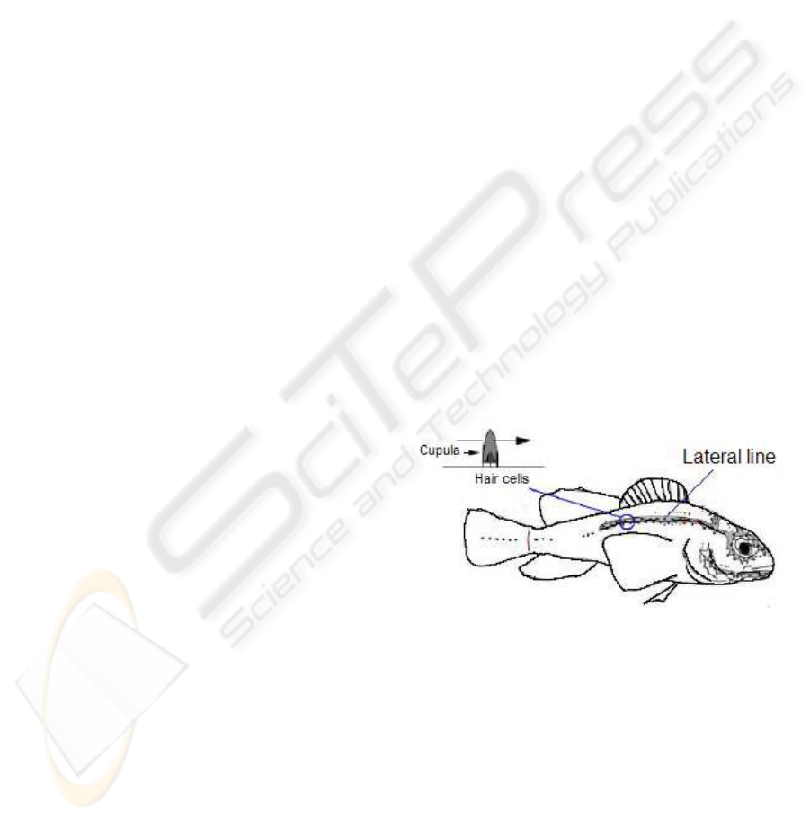
Biologists have discovered that almost all species of
fish have a flow-sensing system, called the lateral line,
consisting of cilium-like haircell sensors (Figure 1)
(Dijkgraaf, 1963). Each haircell sensor in the lateral
line measures local fluid flow velocity, and fish rely on
their lateral lines to perform a wide range of activities
including schooling, preying, navigation, and preda-
tor avoidance (Pitcher and Wardle, 1976; Coombs,
1994). Studies show that using its lateral lines, a
fish can locate and track an acoustic dipole source
(Coombs and Conley, 1997), which models the back-
and-forth motion of the tail of smaller prey or other
fish.
Inspired by the capability of the fish lateral lines,
we are developing an equivalent engineered system,
an artificial lateral line. Potential applications in-
clude maneuvering Autonomous Underwater Vehi-
cles (AUV), dynamic imaging in an underwater en-
vironment, detecting corrosion or leaks inside pipes,
and detecting and tracking intruders such as swim-
mers or submarines.
Recent advances in Micro-Electro-Mechanical
Figure 1: Hair cell sensor system in fish.
Systems (MEMS) technology make it possible to
build micrometer-scale sensors mimicking the func-
tion and structure of fish lateral lines. The first MEMS
lateral line consists of a linear array of 16 hotwire
amemometers (Fan et al., 2002). These sensors are
capable of measuring flow magnitude but not direc-
tion. Recently, MEMS haircell flow sensors, which
are sensitive to flow direction, have also been devel-
oped (Chen and Liu, 2003).
Along with development of sensors, signal-
processing algorithms are also required to make a
complete artificial lateral-line sensory system. Pre-
269
Nguyen N., Jones D., Pandya S., Yang Y., Chen N., Tucker C. and Liu C. (2008).
BIOMIMETIC FLOW IMAGING WITH AN ARTIFICIAL FISH LATERAL LINE.
In Proceedings of the First International Conference on Bio-inspired Systems and Signal Processing, pages 269-276
DOI: 10.5220/0001063002690276
Copyright
c
 SciTePress

vious work in this area localizes and tracks an acous-
tic source using a ML estimator (Pandya et al., 2006)
and introduces a new method for imaging all flow
sources surrounding a sensor array (Pandya et al.,
2007). In this paper, we extend the work in (Pandya
et al., 2007) to cover mapping in three-dimentional
space (3D imaging). In particular, we review the
dipole model and modify the beamforming algorithm
in (Pandya et al., 2007) to handle 3D imaging of
dipoles using haircell sensors. Next, we present a
self-calibration algorithm to adjust the gains across
the sensors to improve estimation accuracy. Finally,
we derive the Cramer-Rao Lower Bound (CRLB) for
the dipole position estimate to find the fundamental
performance limits of the system.
2 ARTIFICIAL LATERAL-LINE
SENSORS
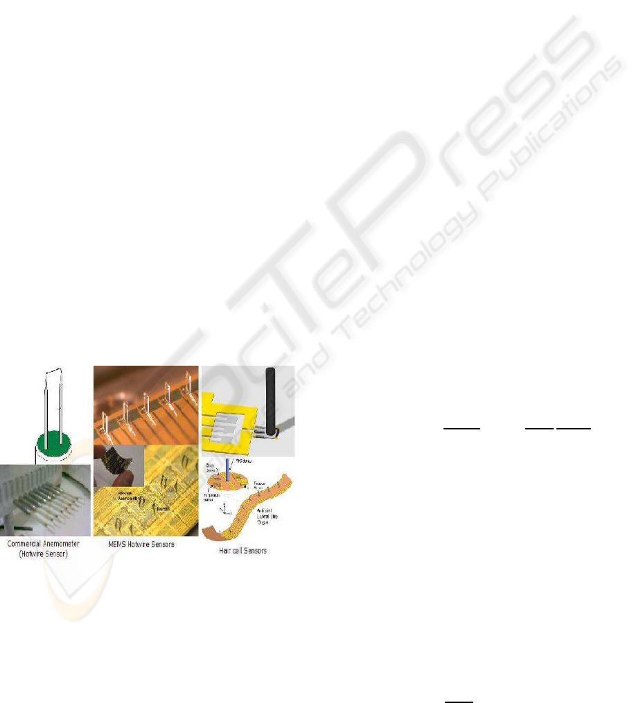
We have used three types of flow sensors to build arti-
ficial lateral lines: conventional hot-wire sensors, mi-
cromachined (MEMS) hot-wire sensors, and hair-cell
sensors (Figure 2). Both types of hot-wire sensors
operate on the heat dissipation principle. Voltage ap-
plied across a sensor heats up the wire. Movement of
water or air particles across the hot wire carries away
heat causing a change in the wire’s resistance and in
turn the current. The change in current reflects the
speed of water or air particles moving across the wire.
Figure 2: Three types of flow sensors for underwater acous-
tic signals.
Conventional hotwire sensors are bulky and
costly. This makes it hard to form small and dense
arrays of sensors for artificial lateral lines. To over-
come those drawbacks, micromachined hotwire sen-
sors have been developed (Chen et al., 2003). They
can be integrated to form a lateral line in a canal as
in fish or to form a dense array of sensors with 1mm
spacing . However, the sensors are fragile and cannot
distinguish the direction of flow. To avoid these prob-
lems, micromachined haircell sensors were invented
that operate on the same principle as in fish. The hair
of the sensor intercepts the flow, and the force applied
on the hair is transformed into stress at the base of the
hair. A piezo-electric strain gauge on a cantilever at
the base translates the stress into an electronic signal
(Yang et al., 2007). The advantages of the haircell
sensors are robustness and directional sensing capa-
bility.
3 FLOW IMAGING USING A
BEAMFORMING APPROACH
Our main goal is to estimate the locations of dipole
sources using arrays of flow sensors in an underwater
environment. In our laboratory experiment, the dipole
source is a small sphere oscillating back and forth in a
certain direction at a fixed frequency. We start with a
dipole source since it is simple enough so that its sur-
rounding flow field model is well established. More-
over, dipole-like flow sources are commonly encoun-
tered in nature, such as the waving tail of a fish. Bi-
ologists have extensively studied fish lateral-line re-
sponse to acoustic dipoles and found that fish can lo-
cate the source of a dipole and track its movement,
and at least some species treat it as prey (Coombs,
1994).
A model of an oscillating dipole source in fluid
has been well studied in (Coombs, 2003). The flow
velocity at a point in space near a dipole source is
modeled as
~v
flow
(r,θ) =

a
3
U
o
cos(θ)
r
3

ˆ
r+

a
3
U
o
2
sin(θ)
r
3

ˆ
θ.
(1)
In the above equation, the flow velocity is a function
of the dipole diameter a, the initial vibrational veloc-
ity amplitude U
o
, and the observation distance r and
angle θ as shown in Figure 3a. Also,
ˆ
r and
ˆ
θ are
unit vectors of the dipole’s spherical coordinates at
the sensor’s position.
The flow velocity in Equation (1) is, however,
derived in the dipole’s spherical coordinates. It is
more convenientto compute flow velocity in the fish’s
Cartesian coordinates (Figure 3b) so that we can de-
rive array patterns due to a dipole oscillating in a cer-
tain direction at some location in space. Transformed
into the fish’s Cartesian coordinates, the flow velocity
is then
~v
flow
(~s) =
a
3
U
o
2r
3
(3cos(θ)
ˆ
r−
ˆ
z
d
) (2)
BIOSIGNALS 2008 - International Conference on Bio-inspired Systems and Signal Processing
270

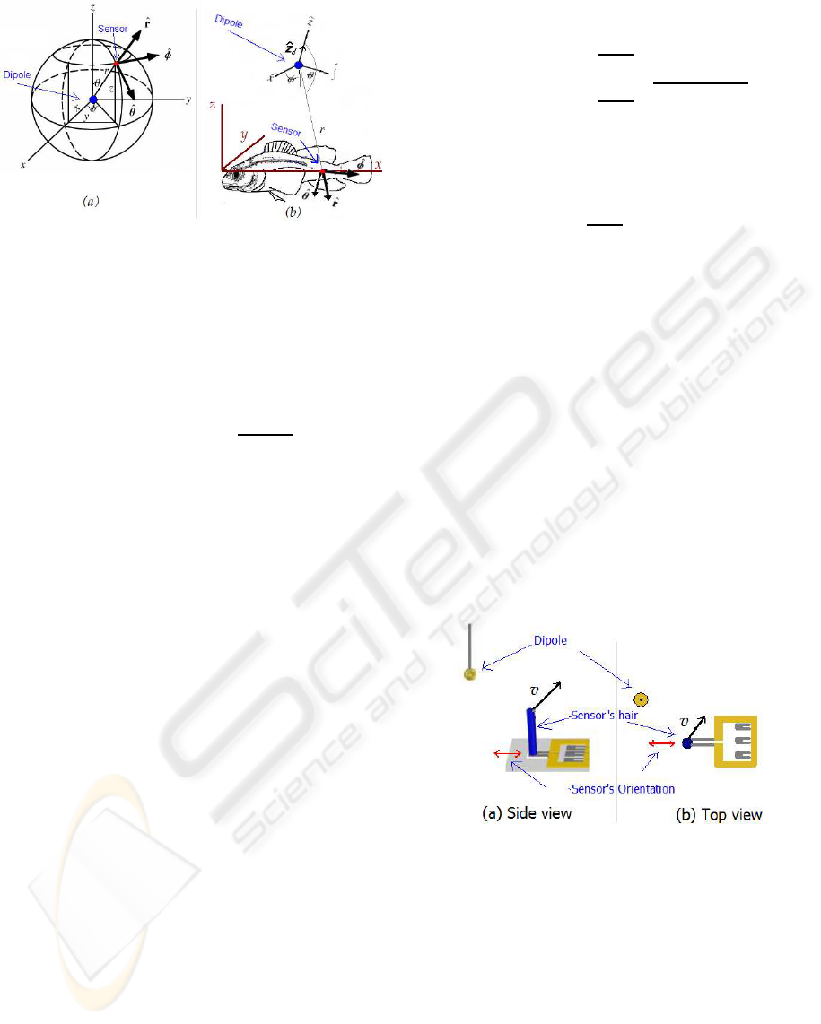
Figure 3: (a) Dipole’s Spherical coodinates. (b) Fish’s
Cartesian coordinates.
where
ˆ
z
d
is now the unit vector on the oscillating axis
of the dipole and~s = (x
s
,y
s
,z
s
) is the vector represent-
ing the position of the sensor in the fish’s coordinates.
If
~
d = (x
d
,y
d
,z
d
) is the vector that indicates the posi-
tion of the dipole, then
r = k~s−
~
dk and
ˆ
r =
~s−
~
d
k~s−
~
dk
Researchers have studied how the lateral lines in
fish respond to the fluid-flow field created by a dipole
source. In (Curcic-Blake and van Netten, 2006), the
excitation patterns along the lateral line of a ruffle
fish (Gymnocephalus cernuus L.) were electrophysio-
logically measured, then compared to theoretical pre-
dictions and found to be in good agreement. The
authors also applied a continuous wavelet transform
(CWT) algorithm on the collected signals to produce
a 2D-contour map of the area surrounding the dipole
source. Although the region of the dipole source
can be identified from the contour map, the map has
poor resolution, making it difficult to visually locate
the dipole’s position or to see multiple simultaneous
sources.
Approaching this problem from the engineer-
ing side, our research group has implemented artifi-
cial lateral lines with both conventional and MEMS
hotwire sensors and used them to capture the sig-
nals in the flow field created by a dipole source. An
adaptivebeamformingapproach using Capon’s beam-
former (Capon, 1969) yielded a much higher resolu-
tion spatial imaging of dipole source then the CWT
(Pandya et al., 2007).
(Curcic-Blake and van Netten, 2006) and (Pandya
et al., 2007) only focus on the case of two-
dimensional imaging. That means that the dipole
source and all the sensors are in the XY-plane, and the
estimation is only concerned with the x and y coordi-
nates. Moreover, (Pandya et al., 2007) used hotwire
sensors that measure flow magnitude, not flow direc-
tion. In this case, the dipole model in Equation (2)
reduces to
k~v
flow
(~s)k =
a
3
U
o
2r
3
k3cos(θ)
ˆ
r−
ˆ
z
d
k
=
a
3
U
o
2r
3
q
3cos
2
(θ) + 1. (3)
In fact, Equation (3) is simplified further when the
dipole’s direction of oscillating
ˆ
z
d
is perpendicular to
XY-plane
k~v
flow
(~s)k =
a
3
U
o
2r
3
since θ = π/2. (4)
Equation (4) is used in (Pandya et al., 2007) to com-
pute expected sensor readings for each position of
dipole in the grid. However, this model no longer
holds when we extend the problem to 3D imaging us-
ing haircell flow sensors.
3.1 3D Imaging with Haircell Sensors
Figure 4 illustrates how the flow velocity ~v
flow
im-
pacts on the hair of an artificial hair cell (AHC) sen-
sor. A dipole source is located above the sensor in
3D space. The flow velocity is computed using Equa-
tion (2). Note that flow velocity now can be in any
direction in 3D space. We neglect here any effects
introduced by the structure to which the sensors are
attached. Figure 4a shows the side view of the flow
vector and Figure 4b shows the top view of it.
Figure 4: (a) Side view of sensor and dipole. (b) Top view
of sensor and dipole.
A single AHC sensor can only measure flow par-
allel with the strain-guage cantilever. Therefore, an
AHC sensor does not measure the magnitude and di-
rection of the flow velocity ~v
flow
but measures the
projection of the flow velocity onto the sensor’s ori-
entation axis. The sensors’ orientations are thus es-
sential information to determine the sensor array re-
sponse.
We extend the adaptive beamforming algorithm in
(Pandya et al., 2007) to enable 3D imaging with AHC
sensors via the steps summarized below:
BIOMIMETIC FLOW IMAGING WITH AN ARTIFICIAL FISH LATERAL LINE
271

• Step 1: Compute the expected sensor array pattern
for each dipole position (x
d
,y
d
,z
d
) in the 3D grid.
For each sensor in the array, use Equation (2) to
compute the flow velocity at that sensor, and then
project the flow velocity onto the sensor’s orien-
tation axis. This produces a template of the array
pattern including L sensor readings
s
(x
d
,y
d
,z
d
)
= [s
1
,s
2
,...,s
L
].
Note that the flow velocity in Equation (2) is
determined by the sensor position vector ~s, the
dipole position vector
~
d = (x
d
,y
d
,z
d
), and the
dipole oscillating vector
ˆ
z
d
.
ˆ
z
d
is a unit vector de-
fined by the azimuth angle θ
d
and the zenith angle
φ
d
. So there are in total 5 parameters to define a
dipole, namely x
d
,y
d
,z
d
for position and θ
d
,φ
d
for
oscillating direction.
• Step 2: Compute the outer-product from the sen-
sor samples
R =
1
N
N
∑
n=1
x[n] ∗ x
T
[n]
where x[n] is the discrete-time vector of samples
of the collected signals.
• Step 3: Using Capon’s method, compute the en-
ergy level at each point in the grid
E =
1
s
H
~
d
R
−1
s
~
d
• Step 4: Plot a map of energy level E for each point
in the 3D grid. The high-energy regions in the
map correspond to the dipole sources’ locations.
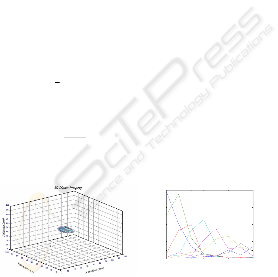
Figure 5: 3D Dipole Imaging with a dipole oscillating at
(50,50,50).
The above algorithm is used in a 3D dipole imag-
ing simulation, and the results are shown in Figure 5.
In this case, we simulate 2 arrays in an L-shape pat-
tern with a total of 21 haircell sensors on the x and
z axes. On each of two axes, there are 11 sensors
spaced 10 mm apart from 0 to 100 mm. A dipole is
located at (50,50,50). Figure 5 shows a sphere cen-
tered around the dipole source with different colour
intensity. High intensity presents the energy level out-
put (from Capon’s formula) at the local point. That
means the dipole is most likely there.
4 SELF-CALIBRATION
ALGORITHM
Calibration of sensors is an important practical step
before doing any signal analysis. Since each individ-
ual sensor’s sensitivity gain can vary (especially for
sensors still in the laboratory stage of development),
poor calibration will lead to poor estimation perfor-
mance. Biological systems have a remarkable abil-
ity to tune their response to environmental variation,
growth, or injury. Self-tuning ability is equally de-
sirable for an engineered system. In this section, we
propose an effective way of doing sensor array cali-
bration for this type of experiment.
A straightforward method for calibration of a sen-
sor array is to sequentially place a dipole in front of
each sensor in the array, then record readings of all the
sensors, which form a series of array patterns. Ideally,
all the patterns should have similar shape and magni-
tude with the peak at the sensor closest to the dipole.
However, measured array patterns vary significantly
due to the non-uniformity of sensor gains. Figure 6
displays an example of the measured array patterns
before calibration.
1 2 3 4 5 6 7 8
0
2
4
6
8
10
12
14
16
Practical sensor array − non−uniform sensor gains
X direction (mm)
Signal strength
Figure 6: Measured sensor array patterns (non-uniform sen-
sor gains).
Mathematically, the calibration problem can be
formulated as follows. Consider a linear array of L
evenly spaced sensors and a series of measurements
BIOSIGNALS 2008 - International Conference on Bio-inspired Systems and Signal Processing
272

as the dipole travels a linear path at a constant dis-
tance from the sensor array. When the dipole is in
front of Sensor 1, the ideal array pattern will be
[s
0
,s
1
,s
2
,...,s
L−1
]
at Sensor 2, it will be [s
−1
,s
0
,s
1
,...,s
L−2
] and so on
until sensor L, [s
−L+1
,s
−L+2
,...,s
0
]. Stacking those
ideal array patterns together produces a Toeplitz ma-
trix
A =












s
0
s
1
s
2
... ... s
L−1
s
−1
s
0
s
1
.
.
.
s
L−2
s
−2
s
−1
.
.
.
.
.
.
.
.
.
.
.
.
.
.
.
.
.
.
.
.
.
.
.
.
s
1
s
2
.
.
.
.
.
.
s
−1
s
0
s
1
s
−(L−1)
... ... s
−2
s
−1
s
0












As each sensor i has a gain g
i
, the matrix of array
patterns with gains is
B =













g
1
s
0
g
2
s
1
g
3
s
2
.. . g
L
s
L−1
g
1
s
−1
g
2
s
0
g
3
s
1
.
.
.
g
L
s
L−2
g
1
s
−2
g
2
s
−1
.
.
.
.
.
.
.
.
.
.
.
.
.
.
.
.
.
.
.
.
.
g
L
s
2
.
.
.
.
.
.
g
(L−1)
s
0
g
L
s
1
g
1
s
−(L−1)
.. . .. . g
(L−1)
s
−1
g
L
s
0













With noise included, the actual readings may be
C = B+ N, where C is the noisy version of B. Figure
6 shows the measured array patterns by plotting the
rows of the matrix C. Although each pattern seems to
have the peak at the sensor closest to the dipole, the
shapes of the patterns are quite different due to non-
uniform sensor gains. The aim of calibration is to find
a set of sensor gains [g
1
,g
2
,...,g
L
] and matrix A that
approximate C as closely, as possible, i.e.
A∗






g
1
0 .. . 0
0 g
2
.
.
.
0
.
.
.
.
.
.
.
.
.
0 ... 0 g
L






≈ C
This is a bilinear least squares problem, which is
a simple special case of a mixed linear-nonlinear least
squares problem (Golub and Pereyra, 1973). Golub
and Pereyra (Golub and Pereyra, 1973) show that
the optimal linear coefficients in the globally optimal
solution are simply the linear least-squares solution
when the nonlinear coefficients are fixed at their glob-
ally optimum values; since the bilinear form is lin-
ear in both the sensor gains g
i
and the shift-invariant
dipole response pattern s
j
when the other is held con-
stant, this holds for both.
We apply the standard iterative solution approach
in which we fix one set of coefficients, find the least-
square optimal solution best fitting the measured data
for the other, and iterate until convergence. (See, for
example, (Bai and Liu, 2006) for recent convergence
theorems for this algorithm for random inputs.) The
algorithm is as follows:
• Step 1: Initialize with uniform gains g
1
= g
2
=
... = g
L
= 1.
• Step 2: Fix the gains [g
1
,g
2
,...,g
L
] and find the
optimal least squares solution for the dipole re-
sponse [s
(−L+1)
,s
(−L+2)
,...,s
0
,...,s
(L−1)
]. This
is equivalent to summing matrix C diagonally and
then dividing it by the sum of all gains corre-
sponding to the column that the diagonal line
crosses.
• Step 3: Fix the dipole response
[s
(−L+1)
,s
(−L+2)
,...,s
0
,...,s
(L−1)
] and find
the optimal least squares solution for the gains
[g
1
,g
2
,...,g
L
]. This is equivalent to summing
up each column of C and dividing it by the
sum of corresponding s
l
that appeared in that
column (see matrix B). For example, after
summing up column 2, it is divided by the sum
(s
1
+ s
0
+ s
−1
+ ... + s
(2−L)
) to get g
2
.
• Step 4: Go back to Step 2 with the new gains in
Step 3. Repeat the process until convergence.
This method allows the on-line calibration of sen-
sors from observation of a dipole source as it travels
across the array. This can be exploited to develop a
fully self-tuning system like biological systems.
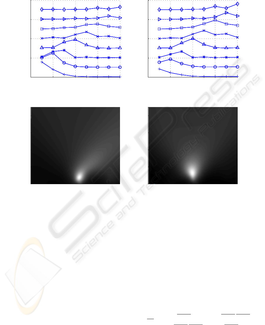
Using the algorithm above, we show the improved
results in Figure 7, using an array of 8 hotwire sensors
positioned 12.5mm apart on the X-axis from 12.5mm
to 100mm. A dipole is placed in front of each sen-
sor and data are collected. Figure 7(A) displays the
array patterns for these eight positions. As can be
seen, these patterns do not look like a shifted version
of each other. The calibration algorithm is applied
to these patterns to produce the calibrated patterns in
Figure 7(B). The improvement in the magnitude and
shape of those patterns is clear. The effect of the cal-
ibration algorithm can be clearly seen as we run a 2D
imaging test of estimating the location of a dipole lo-
cated in front of sensor 4 (50 mm). The image in Fig-
ure 7(C) is the result of processing signals without
calibration while the one in Figure 7(D) uses calibra-
tion. There is obviously a significant improvement in
the accuracy of the image produced by using calibra-
tion.
BIOMIMETIC FLOW IMAGING WITH AN ARTIFICIAL FISH LATERAL LINE
273

0 2 4 6 8
0
20
40
60
80
Array patterns BEFORE calibration
Sensor channels
0 2 4 6 8
0
20
40
60
80
Array patterns AFTER calibration
Sensor channels
0 20 40 60 80 100
0
20
40
60
80
Dipole image WITHOUT calibration
X direction (mm)
Y direction (mm)
0 20 40 60 80 100
0
20
40
60
80
X direction (mm)
Y direction (mm)
Dipole image WITH calibration
(A)
(B)
(C)
(D)
Figure 7: Effects of Self-calibration: (A) Measured array patterns (before calibration), (B) Calibrated array patterns, (C) 2D
dipole imaging without calibration, (D) 2D dipole imaging with calibration.
5 CRAMER-RAO BOUND ON
DIPOLE LOCALIZATION
Fundamental lower bounds on the error of the dipole
position estimate for lateral-line sensors are very use-
ful for evaluation of the estimator presented in Section
3.1, for finding the fundamental performance limit of
a lateral line array, and for evaluating different sensor
array configurations.
The signal captured by sensor k can be modeled
as
s
k
= f
k
(
~
d) + N
k
(5)
where N
k
is the additive Gaussian noise and f
k
(
~
d)
is the expected reading at sensor k produced by a
dipole at location
~
d. For the case of 2D imaging
(
~
d = (x
d
,y
d
)) using hotwire sensors, f
k
(
~
d) is actually
computed by Equation (3); i.e., f
k
(
~
d) = k~v
flow
(~s
k
)k.
For case of 3D imaging using AHC sensors, f
k
(
~
d) is
computed as described in Step 1 of the algorithm in
Section 3.1.
If the noises at all sensors are assumed to be i.i.d.
with zero mean and variance σ
2
N
, the signal vector
of the sensor array s is a Gaussian random vector
N (f(
~
d),Iσ
2
N
). Using the standard procedure in (Poor,
1988), we can derive the Fisher Information Matrix
for the case of 2D imaging as
F =
1
σ
2
N



∑
L
k=1

∂ f
k
(x,y)
∂x

2
∑
L
k=1
∂ f
k
(x,y)
∂x
∂ f
k
(x,y)
∂y
∑
L
k=1
∂ f
k
(x,y)
∂x
∂ f
k
(x,y)
∂y
∑
L
k=1

∂ f
k
(x,y)
∂y

2



(6)
then the CRLB is
Var[
~
d] ≥ [F]
−1
(7)
BIOSIGNALS 2008 - International Conference on Bio-inspired Systems and Signal Processing
274

For the case of 2D imaging using hotwire sensors as
in (Pandya et al., 2007), we have from Equation (3)
f
k
(x,y) =
a
3
U
o
2r
3
=
a
3
U
o
2k~s
k
−
~
dk
3
=
a
3
U
o
2[(x− x
s
k
)
2
+ (y− y
s
k
)
2
]
3
2
then (6) becomes
F =
(
3
2
a
3
U
o
)
2
σ
2
N
×



∑
L
k=1
(x−x
s
k
)
2
[
(x−x
s
k
)
2
+(y−y
s
k
)
2
]
5
∑
L
k=1
(x−x
s
k
)(y−y
s
k
)
[
(x−x
s
k
)
2
+(y−y
s
k
)
2
]
5
∑
L
k=1
(x−x
s
k
)(y−y
s
k
)
[
(x−x
s
k
)
2
+(y−y
s
k
)
2
]
5
∑
L
k=1
(y−y
s
k
)
2
[
(x−x
s
k
)
2
+(y−y
s
k
)
2
]
5



(8)
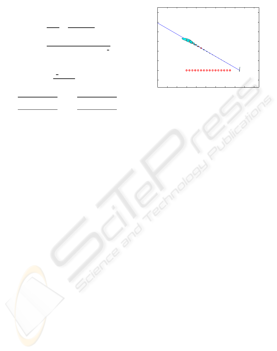
We now compute the CRLB in Equation (8) for a
system consisting of 16 hotwire sensors placed 6mm
apart along the X-axis starting from 60mm to 90mm.
The bounds on the estimation error’s variance are rep-
resented by error ellipses in Figure 8. Each ellipse
corresponds to a dipole located at its center. Note
that the size of the ellipses grows larger as the dipole
moves away from the array. This just agrees with the
fact that as the dipole moves away from the sensor ar-
ray, not only do the signals become weaker but also
the array patterns flatten out. The CRLB shows that
no signal processing algorithm can accurately esti-
mate the location of dipoles at long range (more than
about an array length) because the signals collected
by sensors show almost no difference between dipole
locations.
As the results show, the CLRB can be a source of
design criteria to build a flow sensor array meeting
requirements of image resolution and coverage range.
6 CONCLUSIONS
The adaptive beamforming approach to flow-field
imaging can be generalized to produce an image of
osccilating dipoles’ locations in a three-dimensional
underwater environment. The images’ accuracy in-
creases significantly when a self-calibration algorithm
to tune the sensors’ gains is applied. The calibration
algorithm, which uses the bilinear least squares tech-
nique, is a good starting point to build a system with
the self-tuning capability that biological systems al-
ways exhibit. Our final result, the Cramer-Rao Lower
Bound, is a useful tool to evaluate the performance
limits of a lateral line system. This helps in the de-
sign of a better system. The bounds also confirm that
a lateral-line system is neccessarily a near-field sense.
0 20 40 60 80 100 120 140 160 180 200
−20
0
20
40
60
80
100
120
Error Ellipse for different position of dipole
Axis of sensor array − X direction (mm)
Distance away from array − Y direction (mm)
Figure 8: Error ellipse centered around different dipole po-
sitions, 16 sensors (the circles) are on the x-axis.
ACKNOWLEDGEMENTS
This work was supported by the DARPA BioSenSE
Program under Grant FA-9550-05-1-0459.
REFERENCES
Bai, E. and Liu, Y. (2006). Least squares solutions of bilin-
ear equations. Systems & Control Letters, 55(6):466–
472.
Capon, J. (1969). High-resolution frequency-wavenumber
spectrum analysis. Proceedings of the IEEE,
57(8):1408–1418.
Chen, J., Fan, Z., Zou, J., Engel, J., and Liu, C. (2003).
Two-dimensional micromachined flow sensor array
for fluid mechanics studies. Journal of Aerospace En-
gineering, 16:85.
Chen, J. and Liu, J. (2003). Development of polymer-based
artificial haircell using surface micromachining and
3D assembly. TRANSDUCERS, Solid-State Sensors,
Actuators and Microsystems, 12th International Con-
ference on, 2003, 2.
Coombs, S. (1994). Nearfield detection of dipole sources by
the Goldfish (CARASSIUS AURATUS) and the Mot-
tled Sculpin (COTTUS BAIRDI). Journal of Experi-
mental Biology, 190:109–129.
Coombs, S. (2003). Dipole 3d user guide. Technical report.
Coombs, S. and Conley, R. (1997). Dipole source localiza-
tion by mottled sculpin. I-III. Journal of Comparative
Physiology A: Sensory, Neural, and Behavioral Phys-
iology, 180(4):387–399.
Curcic-Blake, B. and van Netten, S. (2006). Source loca-
tion encoding in the fish lateral line canal. Journal of
Experimental Biology, 209(8):1548–1559.
Dijkgraaf, S. (1963). The functioning and significance of
lateral-line organs. Biology Review, 38:51–105.
BIOMIMETIC FLOW IMAGING WITH AN ARTIFICIAL FISH LATERAL LINE
275

Fan, Z., Chen, J., Zou, J., Bullen, D., Liu, C., and Del-
comyn, F. (2002). Design and fabrication of artificial
lateral line flow sensors. Journal of Micromechanics
and Microengineering, 12(5):655–661.
Golub, G. and Pereyra, V. (1973). The differentiation of
pseudo-inverses and nonlinear least squares problems
whose variables separate. SIAM Journal on Numerical
Analysis, 10(2):413–432.
Pandya, S., Yang, Y., Jones, D., Engel, J., and Liu, C.
(2006). Multisensor processing algorithms for under-
water dipole localization and tracking using MEMS
artificial lateral-line sensors. EURASIP Journal on
Applied Signal Processing.
Pandya, S., Yang, Y., Liu, C., and Jones, D. (2007).
Biomimetic imaging of flow phenomena. Proceed-
ing of Acoustics, Speech and Signal Processing, 2007.
ICASSP 2007, 2:II–933 – II–936.
Pitcher, T. Patridge, B. and Wardle, C. (1976). A blind fish
can school. Science, 194:963–965.
Poor, V. (1988). An Introduction to Signal Detection and
Estimation. Springer-Verlag.
Yang, Y., Chen, N., Tucker, C., Engel, J., Pandya, S., and
Liu, C. (2007). From artificial haircell sensor to artifi-
cial lateral line system: development and application.
MEMS 2007 20th IEEE International Conference on
Micro Electro Mechanical Systems, Kobe, Japan.
BIOSIGNALS 2008 - International Conference on Bio-inspired Systems and Signal Processing
276