MULTIPLE SCALE NEURAL ARCHITECTURE FOR

RECOGNISING COLOURED AND TEXTURED SCENES

Francisco Javier Díaz-Pernas

, Míriam Antón-Rodríguez

, Víctor Iván Serna-González

José Fernando Díez-Higuera

and Mario Martínez-Zarzuela

Department of Signal Theory, Communications and Telematics Engineering, Telecommunications Engineering School

University of Valladolid, Valladolid, Spain

Keywords: Computer Vision, neural classifier, texture recognition, colour image segmentation, Boundary Contour

System, Feature Contour System, ART, colour-opponent processes.

Abstract: A dynamic multiple scale neural model for recognising colour images of textured scenes is proposed. This

model combines colour and textural information to recognise coloured textures through the operation of two

main components: segmentation component formed by the Colour Opponent System (COS) and the

Chromatic Segmentation System (CSS); and recognition component formed by pattern generation stages

and Fuzzy ARTMAP neural network. Firstly, the COS module transforms the RGB chromatic input signals

into a bio-inspired codification system (L, M, S and luminance signals), and then it generates the opponent

channels (black-white, L-M and S-(L+M)). The CSS module incorporates contour extraction, double

opponency mechanisms and diffusion processes in order to generate coherent enhancing regions in colour

image segmentation. These colour region enhancements along with the local textural features of the scene

constitute the recognition pattern to be sent into the Fuzzy ARTMAP network. The structure of the CSS

architecture is based on BCS/FCS systems, thus, maintaining their essential qualities such as illusory

contours extraction, perceptual grouping and discounting the illuminant. But base models have been

extended to allow colour stimuli processing in order to obtain general purpose architecture for image

segmentation with later applications on computer vision and object recognition. Some comparative testing

with other models is included here in order to prove the recognition capabilities of this neural architecture.

1 INTRODUCTION

In biological vision, we can distinguish two main

operating modes: pre-attentive and attentive vision.

The first one performs a parallel and instantaneous

processing which is independent of the number of

patterns being processed, thus covering a large

region of the visual field. Attentive vision,

nevertheless, acts over limited regions of the visual

field (small aperture) establishing a serialised search

by means of focal attention (Julesz & Bergen, 1987).

The proposed model works on the pre-attentive

and attentive mode: pre-attentive segmentation and

attentive recognition. In the pre-attentive process,

the network processes, in a consistent way, colour

and textural information for enhancing regions and

extracting perceptual boundaries to form up the

segmented image. In the attentive mode, the model

merges textural information and the intensity of the

region enhancement in order to punctually recognise

scenes that include complex textures, both natural

and artificial.

The skill of identifying, grouping and

distinguishing among textures and colours is

inherent to the human visual system. For the last few

years many techniques and models have been

proposed in the area of textures and colour analysis

(Gonzalez & Woods, 2002), resulting in a detailed

characterisation of both parameters as well as certain

rules that model their nature. Many of these

initiatives, however, have used geometric models,

omitting the human vision physiologic base and so,

wasting the context dependence. A clear example of

such a feature is the illusory contour formation, in

which context data is used to complete (Grossberg,

1984) the received information, which is partial or

incomplete in many cases.

The architecture described in this work extracts

both colour and textural features from a scene,

segments it into textural regions and brings this

information to an ART classifier, which categorizes

177

Javier Díaz-Pernas F., Antón-Rodríguez M., Iván Serna-González V., Fernando Díez-Higuera J. and Martínez-Zarzuela M. (2008).

MULTIPLE SCALE NEURAL ARCHITECTURE FOR RECOGNISING COLOURED AND TEXTURED SCENES.

In Proceedings of the First International Conference on Bio-inspired Systems and Signal Processing, pages 177-184

DOI: 10.5220/0001063101770184

 SciTePress

the textures using a biologically-motivated learning

algorithm. Humans learn to discriminate textures by

looking at them and becoming sensitive to their

statistical properties in small regions (Grossberg and

Williamson, 1999).

The proposed neural model architecture is based

on the later version of BCS/FCS neural model

(Grossberg et al., 1995; Mingolla et al., 1999), and

on the Fuzzy ARTMAP recognition architecture

(Carpenter et al., 1992). The BCS/FCS model

suggests a neural dynamics for perceptual

segmentation of monochromatic visual stimuli and

offers a multiple scale unified analysis process for

different data referring to monocular perception,

grouping, textural segmentation and illusory figures

perception. The BCS system obtains a map of image

contours based on contrast detection processes,

whereas the FCS performs diffusion processes with

luminance filling-in within those regions limited by

high contour activities. Consequently, regions that

show certain homogeneity and are globally

independent are intensified.

In pre-processing, the main improvement

introduced to the BCS/FCS original model hereby in

this paper, resides in offering a complete colour

image processing neural architecture for extracting

contours and enhancing the homogeneous areas in a

colour image. In order to do this, the neural

architecture develops processing stages, coming

from the original RGB image up to the segmentation

level, following analogous behaviours to those of the

early mammalian visual system. This adaptation has

been performed by trying to preserve the original

BCS/FCS model structure and its qualities,

establishing a parallelism among different visual

information channels and modelling physiological

behaviours of the visual system processes.

Therefore, the envisaged region enhancement is

based on the feature extraction and perceptual

grouping of region points with similar and

distinctive values of luminance, colour, texture and

shading information.

The adaptive categorization and predictive

theory is called Adaptive Resonance Theory, ART.

ART models are capable of stably self-organizing

their recognition codes using either unsupervised or

supervised incremental learning (Carpenter et al.,

1991). ARTMAP theory extends the ART designs to

include supervised learning. Fuzzy ARTMAP

architecture falls into this supervised theory. In

Fuzzy ARTMAP, the ART chosen categories learn

to make predictions which take the form of

mappings to the names of output classes. And thus

many categories can map the same output name.

In section 2, each of the stages composing the

architecture will be explained. Afterwards, section 3

studies its performance over input images presenting

complex textures in order to, in section 4, establish

the conclusions of the analysis and finally assess the

validity of the model depicted here.

2 PROPOSED NEURAL MODEL

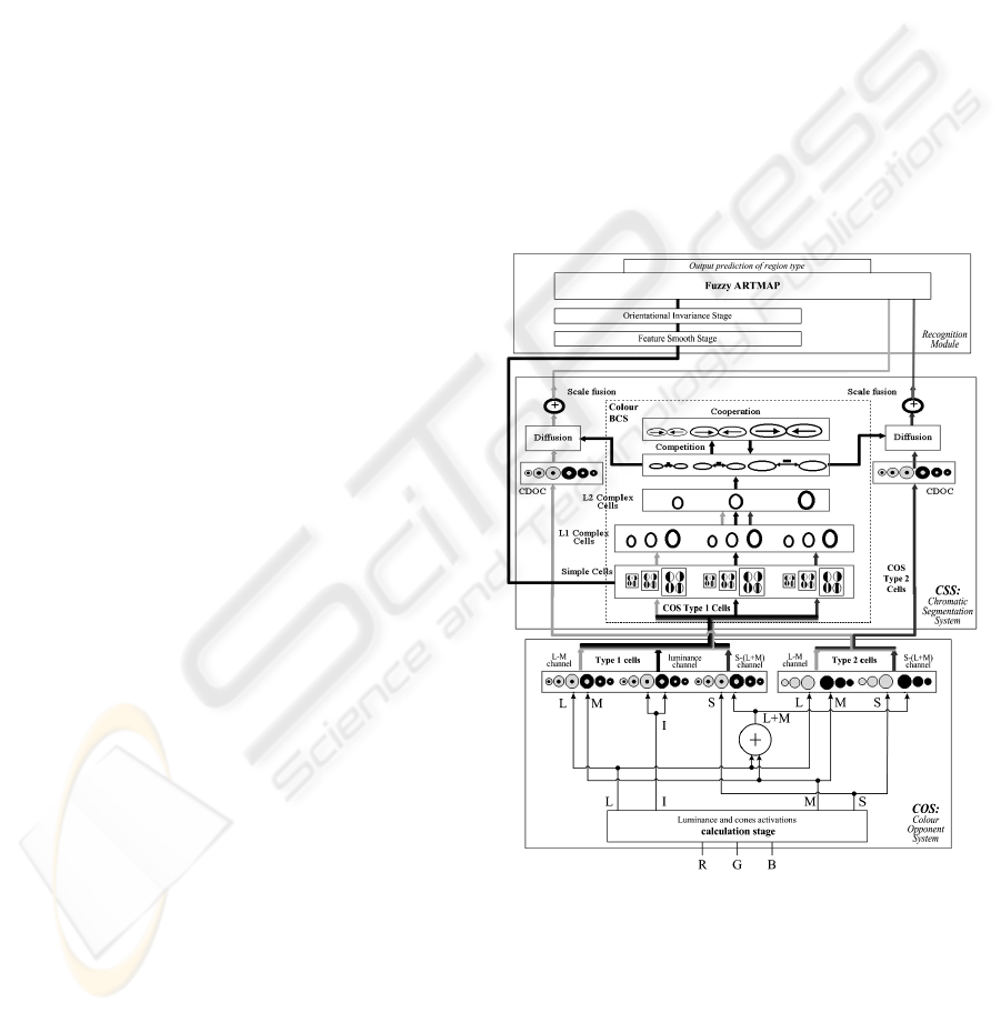
The architecture of the proposed model (Figure 1) is

composed of two main components, colour

segmentation module and recognition module. The

first component consists of two systems called

Colour Opponent System (COS) and Chromatic

Segmentation System (CSS). The recognition

module is made up by a feature smooth stage, an

orientational invariances stage, and a Fuzzy

ARTMAP neural network.

Figure 1: Proposed model architecture. At the bottom, the

detailed COS module structure: on the left, it shows type 1

cells whereas on the right, elements correspond to type 2

opponent cells. In the middle, the detailed structure of the

Chromatic Segmentation System (CSS) based on the

BCS/FCS model. At the top, the recognition module,

based on a Fuzzy ARTMAP network.

The COS module transforms the chromatic

components of the input signals (RGB) into a bio-

BIOSIGNALS 2008 - International Conference on Bio-inspired Systems and Signal Processing

178

inspired codification system, made up of two

opponent chromatic channels, L-M and S-(L+M),

and an achromatic channel.

Resulting signals from COS are used as inputs

for the CSS module where the contour map

extraction and two intensified region images

corresponding to the enhancement of L-M and S-

(L+M) opponent chromatic channels are generated

in multiple scale processing, according to various

perceptual mechanisms (perceptual grouping,

illusory contours, discounting the illuminant and

emergent features). The two enhanced images along

with the textural response from the simple cells form

up the punctual pattern of features that will be sent

to the recognition module where the Fuzzy

ARTMAP architecture generates a context-sensitive

classification of local patterns. The final output of

the proposed neural architecture is a prediction class

image where each point is associated to the texture

class label which it belongs to.

2.1 Colour Opponent System (COS)

The COS module performs colour opponent

processes based on opponent mechanisms that are

present on the retina and on the LGN of the

mammalian visual system (Hubel, 1995). Firstly,

luminance (I signal) and activations of the long (L

signal), middle (M signal), short (S signal)

wavelength cones and (L+M) channel activation (Y

signal) are generated from R, G and B input signals.

The luminance signal (I) is computed as a weighted

sum (Gonzalez & Woods, 2002); the L, M and S

signals are obtained as the transformation matrix

(Hubel & Livingstone, 1990).

In the COS stage, two kinds of cells are

suggested, called type 1 and type 2 cells (see Figure

). These follow opponent profiles intended for

detecting contours (type 1, simple opponency) and

colour diffusion (type 2 cells initiate double

opponent processes).

2.1.1 Type 1 Opponent Cells

Type 1 opponent cells perform two opponent L-M,

S-(L+M), and luminance (Wh-Bl) channels (see

Figure 1). These cells are modelled through two

centre-surround multiple scale competitive

networks, and form the ON and OFF channels

composed of ON-centre OFF-surround and OFF-

centre ON-surround competitive fields, respectively.

These competitive processes establish a gain control

network over the inputs from chromatic and

luminance channels, maintaining the sensibility of

cells to contrasts, compensating variable

illumination, and normalizing image intensity

(Grossberg & Mingolla, 1988). The equations

governing the activation of type 1 cells ((1) and (2))

have been taken from the Contrast Enhancement

Stage in the original models (Grossberg et al., 1995;

Mingolla et al., 1999), but adapted to compute

colour images. The equations for the ON and OFF

channel are:

⎥

⎦

⎤

⎢

⎣

⎡

−+

SSA

CSBSAD

(1)

−

⎥

⎦

⎤

⎢

⎣

⎡

−+

SSA

BSCSAD

(2)

where A, B, C and D are model parameters,

[w]

=max(w,0) and:

∑

qjpi

GeS

and

∑

qjpi

GeS

(3)

with e

as central signal, e

as peripheral signal

(see Table 1), the superscript g=0,1,2 with suitable

values for the small, medium and large scales. The

weight functions have been defined as normalised

Gaussian functions for central (G

) and peripheral

) connectivity.

Table 1: Inputs of different channels on type 1 opponent

cells.

L-M Opponency S-(L+M) Opp. Luminance

-M

-Y

-Bl

Lij Sij Iij

Mij Yij Iij

2.1.2 Type 2 Opponent Cells

The type 2 opponent cells initiate the double

opponent process that take place in superior level,

chromatic diffusive stages (see Figure 1). The

double opponent mechanisms are fundamental in

human visual colour processing (Hubel, 1995).

The receptive fields of type 2 cells are composed

of a unique Gaussian profile. Two opponent colour

processes occur, corresponding L-M and S-(L+M)

channels. Each opponent process is modelled by a

multiplicative competitive central field, presenting

simultaneously an excitation and an inhibition

caused by different types of cone signals (L, M, S

and Y as sum of L and M). These processes are

applied over three different spatial scales in the

multiple scale model shown. Equations (4) and (5)

model the behaviour of these cells, ON and OFF

channels, respectively.

MULTIPLE SCALE NEURAL ARCHITECTURE FOR RECOGNISING COLOURED AND TEXTURED SCENES

179

AD BS

⎡⎤

⎢⎥

⎣⎦

(4)

AD BS

−−

−

⎡⎤

⎢⎥

⎣⎦

(5)

where A, B, C and D are model parameters,

[w]

=max(w,0) and:

(

)

∑

++++

−=

qjpiqjpi

eeGS

)2(

)1(

(6)

(

)

∑

++++

−

−=

qjpiqjpi

eeGS

)1(

)2(

(7)

() ( )

()

ij pq ipjq ipjq

SGee

++ ++

∑

(8)

with e

(1)

and e

(2)

being the input signals of the

opponent process (see Table 2). The weight

functions have been defined as normalised

Gaussians with different central connectivity (G

)

for the different spatial scales g=0, 1, 2:

Table 2: Inputs for different type 2 cells channels.

L-M Opponency S-(L+M) Opponency

-M

-Y

(1)

Lij Sij

(2)

Mij Yij

2.2 Chromatic Segmentation System

(CSS)

As previously mentioned, the Chromatic

Segmentation System bases its structure on the

modified BCS/FCS model (Grossberg et al., 1995;

Mingolla et al., 1999), adapting its functionality to

chromatic opponent signals, for colour image

processing. The detailed structure of CSS can be

seen in Figure 1.

The CSS module consists of the Colour BCS

stage and two chromatic diffusive stages, processing

one chromatic channel each.

2.2.1 Colour BCS Stage

The Colour BCS stage constitutes our colour

extension of the original BCS model. It processes

visual information from three parallel channels, two

chromatic and a luminance channels to obtain a

unified contour map. Analogous to the original

model, the Colour BCS module has two

differentiated phases: the first one (simple and

complex cells) extracts real contours from the output

signals of the COS and the second is represented by

a competition and cooperation loop, in which real

contours are completed and refined, thus generating

contour interpolation and illusory contours (see

Figure 1). Colour BCS preserves all of the original

model perceptual characteristics such as perceptual

grouping, emergent features and illusory perception.

The achieved output coming from the

competition stage is a contour map and it will act as

a control signal serving as a barrier in chromatic

diffusions.

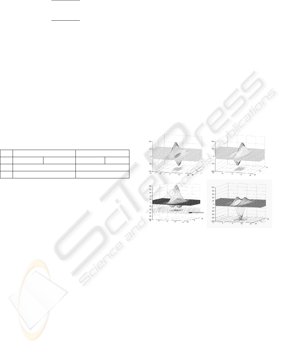
The simple cells are in charge of extracting real

contours from each of the chromatic and luminance

channels. In this stage, the filters from the original

model have been replaced by two pairs of Gabor

filters with opposite polarity, due to their high

sensibility to orientation, spatial frequency and

position (Daugman, 1980). Their presence has been

proved on the simple cells situated at V1 area of

visual cortex (Pollen & Ronner, 1983). Figure 2

shows a visual representation of Gabor filter pair

profiles.

Figure 2: Receptive fields of the filters used to model

simple cells. Top-left: Anti-symmetric light-dark receptive

field. Top-right: Anti-symmetric dark-light receptive field.

Bottom-left: Symmetric receptive field with central

excitation. Bottom-right: Symmetric receptive field with

central inhibition.

The complex cell stage, using two cellular layers,

fuses information from simple cells giving rise to a

final map which contains real contours for each of

the three scales used (see Figure 1).

Detected real contours are passed into a

cooperative-competitive loop, as it is shown in

Figure 1. This nonlinear feedback network detects,

regulates, and completes boundaries into globally

consistent contrast positions and orientations, while

it suppresses activations from redundant and less

important contours, thus eliminating image noise.

The loop completes the real contours in a consistent

way generating, as a result, the illusory contours. In

order to achieve this feature it makes use of a short-

BIOSIGNALS 2008 - International Conference on Bio-inspired Systems and Signal Processing

180

range competition, and a long-range cooperation

stage (Grossberg et al., 1995; Mingolla et al., 1999).

Cooperation is carried out by dipole cells. Dipole

cells act like long-range statistical AND gates,

providing active responses if they perceive enough

activity over both dipole receptive fields lobes (left

and right). Thus, this module performs a long-range

orientation-dependent cooperation in such a way that

dipole cells are excited by collinear (or close to

collinearity) competition outputs and inhibited by

perpendicularly oriented cells. This property is

known as spatial impermeability and prevents

boundary completions towards regions containing

substantial amounts of perpendicular or oblique

contours (Grossberg et al., 1995). The equations

used in competitive and cooperative stages are taken

from the original model (Grossberg et al., 1995).

2.2.2 Chromatic Diffusive Stages

As mentioned above, the chromatic diffusion stage

has undergone changes that entailed the introduction

of Chromatic Double Opponency Cells (CDOC),

resulting in a new stage in the segmentation process.

CDOC stage models chromatic double opponent

cells. The model for these cells has the same

receptive field as COS type 1 opponent cells (centre-

surround competition), but their behaviour is quite a

lot more complex since they are highly sensitive to

chromatic contrasts. Double opponent cell receptive

fields are excited on their central region by COS

type 2 opponent cells, and are inhibited by the same

cell type. We apply double opponency to the L-M

and S-Y channels. This is to say, we apply a greater

sensibility to contrast as well as a more correct

attenuation toward illumination effects, therefore

bringing a positive solution to the noise-saturation

dilemma.

The mathematical model that governs the

behaviour of chromatic double opponent cells is the

one defined by (1) and successive equations, by

varying only their inputs. These inputs are now

constituted by the outputs of the COS type 2

opponent cells for each chromatic channel (see

Table 3).

Table 3: Inputs of the included Chromatic Double

Opponent Cells.

L-M Opponency S-(L+M) Opponency

-M

-Y

-M

)

-M

)

-Y

)

-Y

)

-M

)

-M

)

-Y

)

-Y

)

Chromatic diffusion stages perform four nonlinear

and independent diffusions for L-M (ON and OFF)

and S-Y (ON and OFF) chromatic channels. These

diffusions are controlled by means of a final contour

map obtained from the competition stage while the

outputs of CDOC are the signals being diffused.

At this stage, each spatial position diffuses its

chromatic features in all directions except those in

which a boundary is detected. By means of this

process, image regions that are surrounded by closed

boundaries tend to obtain uniform chromatic

features, even in noise presence, and therefore

producing the enhancement of the regions detected

in the image. The equations that model the diffusive

filling-in can be found in (Grossberg et al., 1995).

As in previous stages, diffusion is independently

performed over three spatial scales in an iterative

manner, obtaining new results from previous

excitations, simulating a liquid expansion over a

surface.

Scale fusion constitutes the last stage of this pre-

processing architecture. A simple linear combination

of the three scales, see equation (9), obtains suitable

visual results at this point.

01 02 11 12

21 22

()()

()

ij ij ij ij ij

ij ij

VAF F AF F

AF F

=−+−

+−

(9)

where A

and A

are linear combination

parameters,

F represents diffusion outputs, with

g indicating the spatial scale (g=0,1,2) and t

denoting the diffused double opponent cell, 1 for ON

and 2 for OFF.

2.3 Recognition Module

The attentive recognition process generates a pattern

by merging the textural response information

coming from the simple cells and the diffusion

intensities of the chromatic channels from the scale

fusion stage. The assorted pattern will be made up

with the responses from the three scales of the

receptive fields, small, medium, and large, the k

orientations, and its two last components being the

chromatic diffusion intensities from the scale fusion

stage of L-M and S-(L+M) channels. Thus a n-

dimensional pattern from each point of the scene

will be created and sent to the Fuzzy ARTMAP

architecture to be learned in the supervised training

process or be categorized in the prediction process.

The ART architecture must learn a mapping from

the input space populated by these feature vectors to

a discrete output space of associated region class

labels. The architecture’s output corresponds with an

image of the class prediction labels in each point.

The recognition stage is composed of three

components: texture feature smooth stage,

MULTIPLE SCALE NEURAL ARCHITECTURE FOR RECOGNISING COLOURED AND TEXTURED SCENES

181

orientational invariances stage, and the Fuzzy

ARTMAP neural network stage.

2.3.1 Texture Feature Smooth Stage

Due to the high spatial variability shown in Gabor’s

filters response a smooth stage is proposed through a

Gaussian Kernel convolution with σ

smooth

deviation,

in all orientations.

2.3.2 Orientational Invariance Stage

In the pattern categorization process some

orientational invariances are generated by means of

the group displacement of components following the

pattern’s existing orientations.

The two last components from diffusion do not

participate in this displacement. Thanks to these

invariances it’s achieved that the same texture

pattern may be viewed from different angles.

3 TESTS AND RESULTS

This section introduces our tests’ simulations over

the proposed architecture.

The recognition process takes place by

generating patterns in every position of the scene,

obtaining them from the outputs of the simple cells.

Those patterns contain textural and colour

information. The textural information for pattern

generation is obtained of the luminance channel. The

colour information is included in the diffusion

components inserted into the pattern.

In order to shape the patterns, the responses

coming from two simple cells filters are used, the

Anti-symmetric light-dark receptive field and the

Symmetric receptive field with central excitation

(see Figure 2). With them, we used three spatial

scales y four orientations. Thus, obtaining a 24-

dimensional textural vector, which, with the two

intensities coming from the scale fusion stage,

generate a 26-dimensional pattern to use as input to

the recognition stage.

In order to show processing nature of the

depicted model, its responses will be analysed and

compared versus other methods, using images which

include complex textures. We begin with a first test

“two textures problem”. The textures image (see

Figure 3a) is composed of two near-regular textures

(weave and brick) which are widely used in texture

benchmarks (Grossberg and Williamson, 1999).

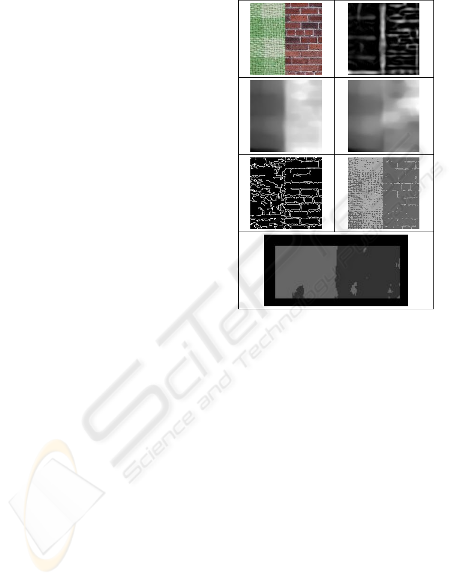
Figure 3: Images of the “two textures test”. a) Original

image, 128x128 pixels. b) Image of the contours map for

large scale, c) Output of the scale fusion stage for the L-M

channel, d) Output of the scale fusion stage for the S-

(L+M) channel, e) Image of extracted contours using

Canny’s extractor, f) Image segmentation with a

pyramidal method, g) Classification result of ‘two

textures’ test. The darker grey level corresponds to the

brick texture prediction while the lighter grey level

corresponds to the weave texture prediction.

Figures 3b, 3c and 3d, display the different stage

outputs of the proposed model. Figure 3b includes

the contour map for large scales, Figures 3c and 3d

include the two outputs coming from the diffusion

stages. Those outputs will constitute the last two

components of the recognition patterns. Figure 3e

include the results from the Canny extractor, using

the cvCanny() with 1, 100, and 70 as parameters;

and 3f shows the output of the pyramidal

segmentation using function cvPyrSegmentation()

with 30000, 30000, and 7 as parameters. cvCanny()

and cvPyrSegmentation() are functions from Intel

Computer Vision Library, OpenCv (Intel, 2006).

Comparing the results, it can be clearly observed

that the proposed architecture behaves in a

compatible manner with the human visual system.

The presented system detects a texture boundary

contour map with perceptual behaviour by extracting

BIOSIGNALS 2008 - International Conference on Bio-inspired Systems and Signal Processing

182

the illusory contour which marks off both textures.

The shown model perceptually differentiates two

textures through filling-in processes controlled by

the illusory vertical contour. Those two comparative

methods do not exhibit a concordance with the

Visual System, and so both extraction and

segmentation obtain worse quality visual results.

Another recognition test was run with a two

textures image. A smooth value of σ

smooth

=4.85 was

chosen for the textural patterns, which corresponds

to a 8x8 resolution, that is, each patch of 8x8 pixels

in the input image yields a single pixel in an output

image for each orientation (Grossberg and

Williamson, 1999). The image was divided into

lower and upper parts. The patterns from the lower

half were taken for Fuzzy ARTMAP network

training using a vigilance parameter of 0.95. The

network was then tested using the patterns coming

from the upper half part. In the supervisory process,

the categories created for the patterns on the left

texture (weave) were associated to a class prediction

pictured light grey, while the patterns coming from

the right texture (brick) where associated to another

class prediction depicted in a darker grey.

In the training process as well as in the testing

one a frame of 10 pixels were left without any

processing. In Figure 3g we can see its resulting

class prediction. The errors committed in the upper

half prediction were of 115 points in the left side

(weave texture) and 112 points in the right side

(brick texture) which brings the error toll to a 3.17%

(96.83% of success). Those statistics are of a similar

magnitude to those obtained in (Grossberg and

Williamson, 1999), where a score of 95.7% was

obtained for a texture mosaic test with 5 textures

instead of two like in our case.

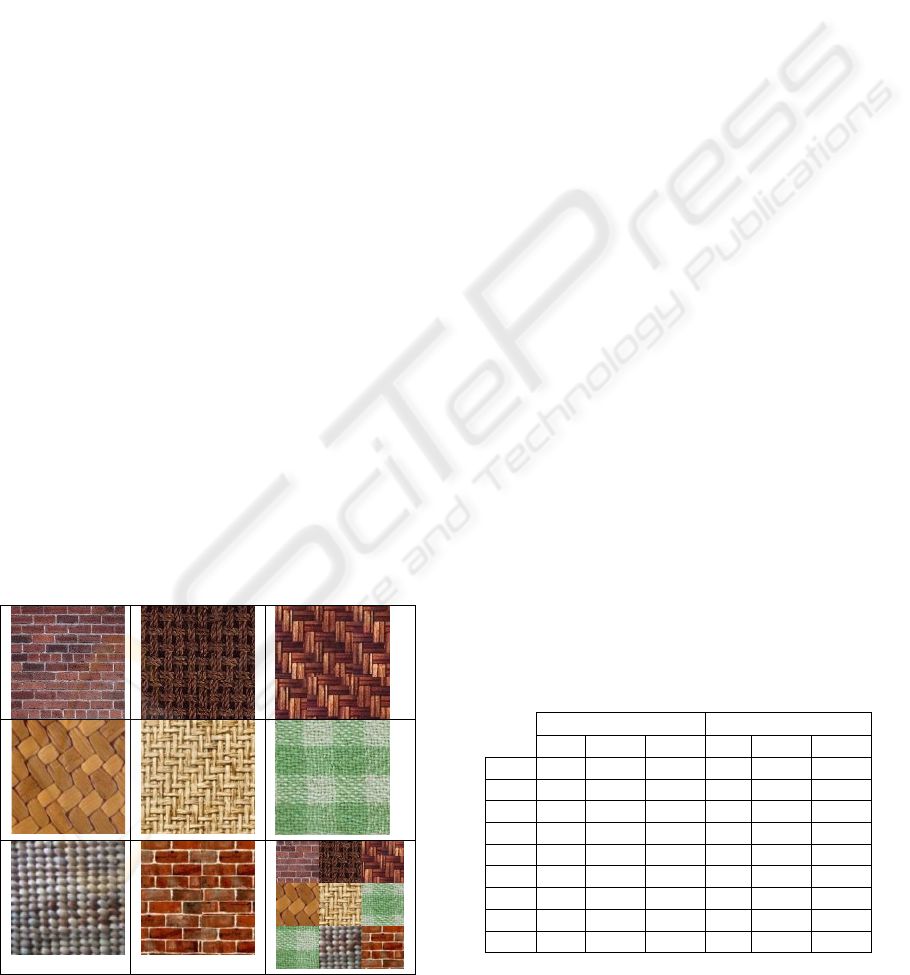
Figure 4: 8-colour texture database (t1 a t8) and multitex

test image.

In order to accomplish this comparison of texture

recognition methods, a test was run, similar to the

“10-texture library problem” proposed in (Grossberg

and Williamson, 1999). We took 8 different classes

of textures with 3 colour images per class (see

Figure 3, only one of each class is presented). Each

texture image consists of 128x128 pixels.

Those 8 classes are included or are of similar

complexity to the black & white image texture

database used in (Grossberg and Williamson, 1999).

Our architecture was trained with points from two of

the images from each class. The training phases

were executed using three different resolutions like

in (Grossberg and Williamson, 1999), 8x8, 16x16,

and 32x32. The third image from each class was

used to evaluate the prediction level of our

architecture. Both training and testing was

performed with two different levels of vigilance,

ρ=0.95 and ρ=0.98 for training and ρ=0.9 and

ρ=0.97, respectively for testing. The results are

shown in Table 4, where the statistics for each class

of texture are depicted. It can be observed that the

success rate of the predictions increase with low

resolutions. The global results are shown in the last

row of Table 4. Our recognition system achieved

96,4%, 98.0% and 97.4% corrects with ρ=0.95; and

98.0%, 99.6% and 97.4% corrects with ρ=0.98 in

8x8, 16x16 and 32x32 resolution, respectively. The

ARTEX system proposed in (Grossberg and

Williamson, 1999) achieved worse results in the two

first resolutions. ARTEX system achieved 95.8%,

97.2% and 100.0% corrects with all its features and

one training epoch (no information about the

vigilance parameter is given). In Table 4, it can be

seen that the first texture sharply decreases the

success rate because it is a highly irregular (no

regular brick size and colour). The others statistical

values are over those obtained by ARTEX system.

Table 4: 8-textures recognition statistics for each texture

class and global.

ρ=0.95 ρ=0.98

8x8 16x16 32x32 8x8 16x16 32x32

90.0 86.9 80.3 90.9 87.2 79.3

97.3 100 100 97.1 100 100

98.1 98.5 99.0 98.8 99.8 100

98.7 99.8 99.8 99.9 100 100

97.8 100 100 99.2 100 100

99.9 99.9 100 100 100 100

97.6 100 100 99.9 100 100

92.1 98.5 100 98.4 100 100

total

96.4 98.0 97.4 98.0 99.6 97.4

Our architecture was also trained and tested over

a “multitex problem”, analog but more complex than

MULTIPLE SCALE NEURAL ARCHITECTURE FOR RECOGNISING COLOURED AND TEXTURED SCENES

183

the “texture mosaic problem” proposed in

(Grossberg and Williamson, 1999). Our mosaic

includes 9 textural areas versus the 5 textural areas

from (Grossberg and Williamson, 1999). As

explained before, with the third image from each

texture class, we built a 210x210 pixels multitex test

image (see Figure 4 row 3-right) in order to evaluate

the frontier precision between textures in the

prediction of our architecture. Both the training and

the testing was performed with two different levels

of vigilance, ρ=0.95 and ρ=0.98 for training and

ρ=0.9 and ρ=0.97, respectively for testing. The

results are shown in Table 5. Those results show a

better class rate in all resolutions and vigilance

levels than those obtained in (Grossberg and

Williamson, 1999) as our worst result (95.89%)

beats the best result (95.7%) shown in this work.

Table 5: Multitex prediction statistics.

Resolution Train vigilance

parameter

Samples

/class

Class rate

(%)

8x8 0.95 300

95.89

16x16 0.95 125

96.67

32x32 0.95 40

97.30

8x8 0.98 300

99.75

16x16 0.98 125

99.48

32x32 0.98 40

99.18

The images of the predictions can be seen in

Figure 5 where only those corresponding to a

vigilance parameter value of ρ=0.95 are shown.

Each prediction class is depicted with a level of

grey, from black to white. Those images reveal two

remarkable points. First, the best prediction for the

interior points shows up for a 32x32 resolution.

However, it is the 8x8 resolution the one which

accurately resolve texture transitions.

The main differences between our architecture

and the one shown in (Grossberg and Williamson,

1999) are basically the inclusion of colour

information (the two output signals coming from the

chromatic channels in the diffusion stage) and the

use of one additional receptive field in the pattern’s

textural components. Our architecture also includes

in the patterns the processing of the symetric

receptive field with central excitation simple cells.

REFERENCES

Carpenter, G.A., Grossberg, S., Markuzon, N. and

Reynolds, J.H. (1992). Fuzzy ARTMAP : A Neural

Network Architecture for Incremental Supervised

Learning of Analog Multidimensional Maps. Neural

Networks, 3, 5, 698 -713.

Daugman, J.G. (1980) Two-dimensional spectral analisis

of cortical receptive field profiles. Vision Research,

20, 847-856.

Gonzalez, R.C. and Woods R.E. (2002), Digital Image

Provessing, 2/E, Prentice Hall.

Grossberg, S. (1984). Outline of a theory of brightness,

colour, and form perception. In E. Degreef and J. van

Buggenhault (Eds.) Trends in mathematical

psychology. Amsterdam: North Holland.

Grossberg, S. and Hong, S. (2006). A Neural Model of

Surface Perception: Lightness, Anchoring, and Filling-

In. Spatial Vision, 19, 2, 263-321.

Grossberg, S. and Williamson, J.R. (1999). A self-

organizing neural system for leaning to recognize

textured scenes, Vision Research, 39, pp. 1385-1406.

Grossberg, S., and Mingolla, E. (1988). Neural dynamics

of perceptual grouping: textures, boundaries, and

emergent segmentations. In Grossberg, S. (Ed.): The

adaptive brain II. Chap. 3. Amsterdam, North Holland,

1988.

Grossberg, S., Mingolla, E. and Williamson, J. (1995).

Synthethic aperture radar processing by a multiple

scale neural system for boundary and surface

representation. Neural Networks, 8, 1005-1028.

Hubel D.H. (1995) Eye, Brain and Vision. Scientific

American Library, No. 22., WH Freeman, NY. p. 70.

Hubel, D.H., and Livingstone, M.S. (1990). Color and

contrast sensitivity in lateral geniculate body and

Primary Visual Cortex of the Macaque Monkey. The

Journal of Neuroscience, 10, 7, 2223-2237.

Intel Corporation (2006). Open Source Computer Vision

Library. http://www.intel.com/technology/computing/

opencv/

Julesz, B., and Bergen, R. (1987), Textons, The

Fundamental Elements in Preattentive Vision and

Perception of Textures. In Fischer and Firschen (eds.).

Readings in Computer Vision, 243-256, 1987.

Mingolla, E., Ross, W. and Grossberg, S. (1999) A neural

network for enhancing boundaries and surfaces in

synthetic aperture radar images. Neural Networks, 12,

499-511, 1999.

Pollen, D.A. and Ronner, S.F. (1983) Visual cortical

neurons as localized spatial frequency filters. IEEE

Transactions on Systems, Man, and Cybernetics,

SMC-13, No 15, 907-916.

BIOSIGNALS 2008 - International Conference on Bio-inspired Systems and Signal Processing

184