
MEASURING CHANGES OF 3D STRUCTURES IN
HIGH-RESOLUTION µCT IMAGES OF TRABECULAR BONE
Norbert Marwan, J
¨
urgen Kurths
Nonlinear Dynamics Group, Institute of Physics, University of Potsdam, 14415 Potsdam, Germany
Peter Saparin
Department of Biomaterials, Max Planck Institute of Colloids and Interfaces, 14424 Potsdam-Golm, Germany
Jesper S. Thomsen
Department of Biology, Institute of Anatomy, University of Aarhus, 8000
˚
Arhus, Denmark
Keywords:
Measures of complexity, 3D image analysis, structural analysis, trabecular bone, osteoporosis.
Abstract:
The appearances of pathological changes of bone can be various. Determination of apparent bone mineral
density is commonly used for diagnosing bone pathological conditions. However, in the last years the struc-
tural changes of trabecular bone have received more attention because bone densitometry alone cannot explain
all variation in bone strength. The rapid progress in high resolution 3D micro Computed Tomography (µCT)
imaging facilitates the development of new 3D measures of complexity for assessing the spatial architecture
of trabecular bone. We have developed a novel approach which is based on 3D complexity measures in order
to quantify spatial geometrical properties of bone architecture. These measures evaluate different aspects of
organization and complexity of trabecular bone, such as complexity of its surface, node complexity, or local
surface curvature. In order to quantify the differences in the trabecular bone architecture at different stages
of osteoporotic bone loss, the developed complexity measures were applied to 3D data sets acquired by µCT
from human proximal tibiae and lumbar vertebrae. The results obtained by the complexity measures were
compared with results provided by static histomorphometry. We have found clear relationships between the
proposed measures and different aspects of bone architecture assessed by the histomorphometry.
1 INTRODUCTION
Bone is a dynamic tissue that adapts its architecture to
the loading conditions it is subjected to. In addition,
from the third decade of life the amount of bone tis-
sue is gradually decreasing. However, in patients with
osteopenia or osteoporosis or in astronauts staying in
micro-gravity conditions for a long period of time, the
bones may change so dramatic that they will lose a
significant amount of their stability and the fracture
risk increases. These changes may emerge on the one
hand as the loss of bone, a decrease of the mineral-
ization of bone, and on the other hand as a change in
the micro-architecture of the interior spongy part of
the bone called trabecular bone. Structural changes
of trabecular bone have received more attention in the
last years because the bone loss alone cannot explain
all variation in bone strength. Moreover, the rapid
progress in high resolution 3D Micro-Computed To-
mography (µCT) imaging facilitates the investigation
of the micro-architecture of bone.
The standard method for assessing the bone sta-
tus and its micro-architecture is bone histomorphom-
etry, which was developed for 2D (Parfitt et al.,
1983) and recently extended for 3D analysis (Ito
et al., 1998; Hildebrand et al., 1999). More re-
cently developed methods for quantifying the com-
plexity of trabecular structures includes methods us-
ing measures of complexity based on symbolic dy-
namics (Saparin et al., 1998; Saparin et al., 2005),
fractal properties (Marwan et al., 2007b) and on re-
currence (Marwan et al., 2007a), or using volumetric
spatial decompositions (Stauber and M
¨
uller, 2006).
By applying these approaches to 3D images of tra-
becular bone, it was shown that the bone micro-
architecture changes substantially during the devel-
opment of osteopenia/osteoporosis. The main con-
clusions in (Saparin et al., 2005; Marwan et al.,
2007a) were that the complexity of the bone micro-
architecture decreases with increasing bone loss and
that the volume and surface of the trabecular struc-
ture changes in a different amount. This latter conclu-
425
Marwan N., Kurths J., Saparin P. and S. Thomsen J. (2008).
MEASURING CHANGES OF 3D STRUCTURES IN HIGH-RESOLUTION µCT IMAGES OF TRABECULAR BONE.
In Proceedings of the First International Conference on Bio-inspired Systems and Signal Processing, pages 425-430
DOI: 10.5220/0001064004250430
Copyright
c
SciTePress
sion confirms former findings that the shapes of the
trabeculae change during bone loss, e. g., from plate-
like structure to rod-like structure (Hildebrand et al.,
1999).
In this study we develop new measures of com-
plexity for quantifying the shape and the complexity
of 3D structures. We use 3D geometrical properties
like local ratio of bone volume to bone surface and
the local configuration of the neighbourhood of the
bone voxels. We apply these measures to 3D µCT
images of human proximal tibial and vertebral bodies
in order to investigate differences in trabecular bone
structure at different stages of bone loss and compare
the results with the outcome of the histomorphomet-
rical evaluation of the same bone material.
2 MEASURES OF COMPLEXITY
The idea behind the quantification of a geometrical
shape is based on the fact that different 3D objects of
the same volume have different surfaces, depending
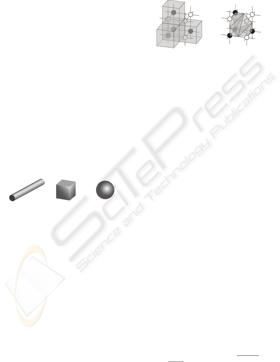
on their geometrical shape. For example, a long cylin-
der (length is much larger than radius) has a larger
surface than a cube of the same volume, and a sphere
of the same volume has a smallest possible surface for
the same given volume (Fig. 1).
Figure 1: Long cylinder, cube and sphere of same volume
(V = 1000) have different surface (S
cylinder
= 694 (for this
arbitrary proportion), S
cube
= 600, S
sphere
= 484).
Based on the relationship between surface and
shape, we introduce measures using the local bone
surface and local bone volume. Surface and volume
of the trabecular bone are locally estimated in a small
cubic box of size s, which moves through the entire
3D image.
Surface and volume could be estimated by a sim-
ple Lego brick approach. The number of voxels form-
ing the bone structure is used as the volume, and the
number of such bone voxels which are connected to
the bone marrow (surface voxels) as the bone sur-
face (Fig. 2A). However, this approach is rather prob-
lematic, because the amount of surface voxels is ac-
tually not a two-dimensional surface measure as it
should be, but a three-dimensional volumetric mea-
sure. Moreover, the bone volume will be overesti-
mated when such a simple voxel counting algorithm
is used. Subsequent calculations based on this sur-
face and volume estimation will lead to even more
erroneous estimations. In order to get more precise
results, we apply an iso-surface algorithm (Fig. 2B).
B
A
Figure 2: A fragment of data consisting of eight voxels in-
cluding four bone voxels (black nodes) and four marrow
voxels (white nodes). In the Lego brick. approach (A), the
surface of bone is estimated by counting the number of bone
voxels which are connected with marrow voxels (the top,
front and right black nodes), and the volume is the number
of all bone voxels. In the iso-surface approach (B), the sur-
face is estimated by the sum of triangles which form an iso-
surface between bone and marrow voxels; the volume is the
sum of the tetrahedrons which can be filled between such
iso-surface and the grid lines. The volume (gray shaded)
will be overestimated by using the Lego brick approach (A),
but will be calculated more precise by using the iso-surface
approach (B).
An appropriate approach to construct iso-surface
is the marching cubes algorithm (Lorensen and Cline,
1987) which is widely used for constructing iso-
surfaces in 3D data visualisation. A marching cube
(MC) consists of eight neighbouring voxels. If two
neighbouring voxels of this MC have voxel val-
ues above and below a predefined threshold value
(i. e. one is bone and another is non-bone voxel), the
iso-surface will lie between these two voxels. In such
MC the iso-surface is formed by a set of triangles,
and the surface estimation is the sum of the areas of
these triangles (Fig. 2B). Now we introduce the same
approach for the estimation of the bone volume. The
bone volume within the MC is filled with tetrahedrons
in such a way, that the resulting surface equals the iso-
surface, which is formed by triangles (Fig. 3). The
sum of the volumes of these tetrahedrons is the esti-
mated bone volume contained in the MC.
For the quantification of the 3D shape, we intro-
duce at first the ratio between the local bone surface
S
bone
and the minimal possible surface of the given
local bone volume V
bone
, which is the surface of a
sphere S
sphere
containing this volume V
bone
. We call
this ratio local shape index σ
loc
. Because the local
bone volume V
bone
depends on the size of the mov-
ing box s, the normalized local bone volume
ˆ
V
bone
=
V
bone
/s
3
is used (
ˆ
V corresponds to the local bone vol-
ume fraction or density BV/TV
loc
). The local shape
index
σ
loc
=
S
bone
S
sphere
with S
sphere
=
3
q
36π
ˆ
V
2
bone
(1)
BIOSIGNALS 2008 - International Conference on Bio-inspired Systems and Signal Processing
426
1
5
2
6
7
3
4
0
Figure 3: Same fragment as shown in Fig. 2, which is also
called marching cube. For volume estimation, the marching
cube is filled with tetrahedrons constructed between the iso-
surface and the grid lines.
distinguishes between different shapes with the same
volume but whose surface differ, like plates and rods.
In principle, the value of this index should be equal or
larger than one, because the surface of a sphere is the
smallest possible surface. However, the object could
be cut by the faces of the moving box; these interfaces
are not counted for the surface of the structure, result-
ing in a smaller surface. This can even result in a sur-
face that is smaller than such of a sphere. However,
this would mainly be the case if the structure is con-
cave. Therefore, values of σ
loc
smaller than one rep-
resent concave structures, whereas values larger than
one represent convex structures.
Because σ
loc
is computed within a small box while
moving through the studied object, we get a frequency
distribution of the shape index over the entire ob-
ject p(σ
loc
). Based on this distribution, the averaged
shape index
A
σ
= hσ
loc
i
VOI
, (2)
which is the average of all σ
loc
in the volume of inter-
est (VOI); it measures the mean shape of the trabecu-
lar structures.
Next we define the shape complexity as the condi-
tional entropy of the joint distribution p(σ
loc
,V
loc
) in
a given bone volume V
loc
C
σ
= −
∑
σ
loc
,V
loc
p(σ
loc
,V
loc
)log
p(σ
loc
,V
loc
)
p(V
loc
)
(3)
This measure quantifies the variety of different shapes
for various bone volumes. If the bone surface changes
in the same manner as the bone volume changes,
i. e. the shape of the structure is roughly remaining,
this measure will be low. If, however, the shape is
changing more dramatically and perhaps irregularly
due to changing bone volume, as it is the case for bone
loss, C
σ
will be high.
As already mentioned, an MC is formed from
eight neighbouring voxels, arranged in the shape of
a cube. The entire VOI is actually a composition of
many such MCs. In each MC, depending on the posi-
tions of the bone voxels, there are 256 configurations
possible; neglecting rotational and inversion symme-
try, there are 15 unique and fundamental MC config-
urations (Lorensen and Cline, 1987). However, we
will only consider rotational symmetry and ignore in-
version, hence, we will deal with 21 pseudo-unique
MC configurations (Fig. 4). A specific marching cube
configuration corresponds to a specific bone surface
configuration and, hence, it is related with the com-
plexity of the surface. For all MCs composing the
VOI we identify and count each MC configuration
and can derive the probability p(MC) with which a
certain MC configuration occurs in the 3D architec-
ture.
MC 0
MC 7
MC 14
MC 11
MC 18
MC 1
MC 15
MC 8
MC 2
MC 9
MC 16
MC 3
MC 10
MC 17
MC 12
MC 19
MC 4
MC 20
MC 5 MC 6
MC 13
Figure 4: The 21 pseudo-unique marching cube configura-
tions used for defining the marching cubes entropy index.
Since these pseudo-unique marching cube config-
urations (MC cases) are related with the surface com-
plexity, we define an additional measure, the march-
ing cubes entropy index
I
MC
= −
∑
MC
p(MC)log p(MC) (4)
which is the Shannon entropy of the probability den-
sity p(MC) of the marching cubes cases; it measures
the complexity of the surface of the trabecular struc-
tures. Simple complex surfaces will result in low val-
ues of I
MC
, whereas complex surfaces will result in
high values of I
MC
.
Note that shape complexity C
σ
and marching
cubes entropy index I
MC
characterises different kinds
of order in a structure. Whereas I
MC
assesses a global
order (or disorder) of bone surfaces, C
σ
quantifies the
order of certain structural shapes depending on the
structure volume. Therefore, these two measures are
not necessarily correlated with each other.
3 MATERIALS
These newly introduced measures, Eqs. (2), (3) and
(4), are used for the assessment of structural changes
MEASURING CHANGES OF 3D STRUCTURES IN HIGH-RESOLUTION µCT IMAGES OF TRABECULAR BONE
427
in trabecular bone due to bone loss in osteoporosis.
29 trabecular bone biopsies from proximal tibia
bone specimens and 18 entire lumbar vertebral bod-
ies L4 were obtained from the same set of donors.
The proximal tibial bone biopsies were scanned at
Scanco Medical AG (Bassersdorf, Switzerland) by
using a Scanco µCT 40 µCT scanner with a voxel size
of 20 µm (Thomsen et al., 2005). The vertebral bod-
ies were scanned at Scanco Medical AG by using a
Scanco µCT 80 with a voxel size of 37 µm. In or-
der to get comparable images for both skeletal sites,
proximal tibia images were downsampled to a voxel
size of 40 µm. The analysed set of specimens includes
normal, osteopenic (initial stage of osteoporosis) and
osteoporotic bones.
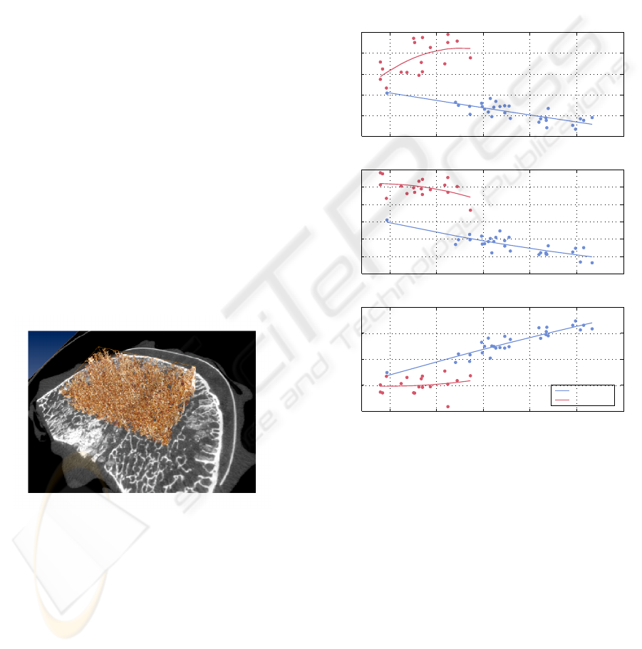
Standardized volumes of interest (VOI) were ap-
plied to the µCT images for quantification of the 3D
architecture: The VOI for the proximal tibial biop-
sies was located 5 mm below the cortical shell and
were 10 mm long, whereas the VOI for the verte-
bra was a 25 × 15 × 10 mm
3
cuboid with the cen-
ter shifted 4.5 mm backwards from the center of the
vertebra along its symmetry line (Fig. 5). The struc-
tural measures of complexity are then computed using
these VOIs. In order to validate the developed mea-
sures, the results of the purposed 3D data evaluation
were compared against conventional bone histomor-
phometry (Thomsen et al., 2000). Histomorphometric
measures are discussed below.
Figure 5: Volume of interest applied to a human lumbar
vertebra. Analysed part of the trabecular structure is shown
in brown, grey-scale image is the axial CT slice through the
middle of the vertebral body.
4 RESULTS
Applying the introduced measures of complexity to
the VOIs within the 3D µCT images, we perform an
evaluation of the micro-architecture of the trabecular
bone of 29 proximal tibial biopsies and 18 lumbar ver-
tebrae representing different stages of bone loss in os-
teoporosis. The size of the moving box was chosen as
20 ×20 × 20 voxels.
At first we study the differences of the trabecu-
lar structure due to bone loss and compare the tra-
becular bone architecture in proximal tibia and lum-
bar vertebra (Fig. 6). Bone volume to total volume
ratio BV/TV (derived from histomorphometry) char-
acterises the amount of bone material and is used as
an indicator of bone loss. We find some remarkable
differences between the proximal tibia and the lumbar
vertebra.
5 10 15 20 25 30
0.8
1
1.2
1.4
1.6
1.8
BV/TV (%)
A
σ
5 10 15 20 25 30
0.3
0.32
0.34
0.36
0.38
0.4
0.42
BV/TV (%)
C
σ
5 10 15 20 25 30
5
5.5
6
6.5
7
BV/TV (%)
I
MC
Tibiae
Vertebrae
Figure 6: Measures of complexity vs. bone loss (repre-
sented by bone volume fraction BV/TV) for proximal tibiae
(blue line) and lumbar vertebrae (red line). The lines are
square-polynomial fits to guide the eye.
During bone loss, A
σ
decreases in the vertebra,
but increases in the proximal tibia. Moreover, for
high density proximal tibiae (BV/TV > 20%) its val-
ues are below one. This suggests that the normal
trabecular bone in proximal tibial contains a large
number of concave structures. Bone loss causes a
shift from concave structures towards convex ones.
A
σ
for vertebra is higher than one. The Spearman’s
rank correlation coefficient between BV/TV and A
σ
is
R = −0.75 (proximal tibia) and R = 0.57 (vertebra).
On a p = 0.01 significance level, the correlation for
the proximal tibia is significant, but for the vertebrae
it is not.
BIOSIGNALS 2008 - International Conference on Bio-inspired Systems and Signal Processing
428
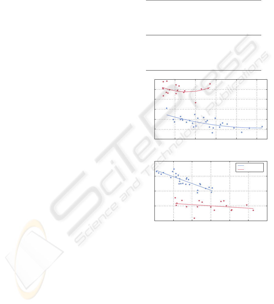
C
σ
reveals the same trend for both proximal tibia
and vertebra. I
MC
reveals also the same trend for both
skeletal sites. However, the direction of the correla-
tions between C
σ
and I
MC
are opposite. The correla-
tions are only significant for the proximal tibia. From
the correlation between I
MC
and BV/TV we infer that
the complexity of the bone surface decreases during
bone loss. The anti-correlation with C
σ
suggests that
the variety of shapes increases during bone loss, as it
is the case when plate-like structures deteriorate to-
wards rod-like structures, or rod-like structures be-
come disconnected.
Next, we compare the introduced structural mea-
sures of complexity with some of the classical histo-
morphometrical measures (Tab. 1, Fig. 7). The ma-
jority of these measures are significantly correlated
to the measures of complexity at the proximal tibia
only. This is probably due to a higher variability of
the shapes in proximal tibia.
The trabecular separation Tb.Sp measures the
mean trabecular plate separation under the assump-
tion that the bone tissue is distributed as parallel plates
(Parfitt et al., 1983). At the vertebral body only A
σ
is significantly correlated with Tb.Sp. At the proxi-
mal tibia both C
σ
and I
MC
are weakly correlated with
Tb.Sp.
The nodes-termini ratio Nd/Tm represents the
connectivity of the network as it appears on a 2D sec-
tion (Garrahan et al., 1986). A change in the connec-
tivity of the network causes a change in the complex-
ity of bone surface. Therefore, at the proximal tibia
we find that Nd/Tm is strongly correlated with I
MC
.
At the vertebral body Nd/Tm and I
MC
are also corre-
lated, but this correlation does not reach the level of
significance.
A further common way to characterise the tra-
becular network is the trabecular bone pattern factor
TBPf (Hahn et al., 1992). It is, like Nd/Tm, strongly
related with the suggested measures of complexity, in
particular with I
MC
. Again, for vertebrae these corre-
lations are not significant.
These results confirm that the averaged shape in-
dex A
σ
, shape complexity C
σ
and marching cubes en-
tropy index I
MC
express the shape and complexity of
the trabecular micro-architecture. The different as-
pects of the introduced measures of complexity are
clearly illustrated at the proximal tibia and by compar-
ing tibia and vertebral trabecular bone architectures.
We proved quantitatively that the architecture of the
trabecular bone of lumbar vertebra is very different
from that of the proximal tibia. This difference is also
clearly emphasised by the new structural measures.
Therefore, we infer that these measures reveal addi-
tional information about the bone structure, which are
Table 1: Spearman’s rank correlation coefficients between
structural measures of complexity and bone volume fraction
as well as histomorphometrical measures. Statistically sig-
nificant values (p = 0.01) are black, non-significant values
are gray.
A
σ
C
σ
I
MC
Proximal Tibiae
BV/TV −0.75 −0.72 0.88
Tb.Sp 0.45 0.58 −0.64
Nd/Tm −0.72 −0.65 0.88
TBPf 0.72 0.66 −0.90
Lumbar Vertebrae
BV/TV 0.57 −0.27 0.25
Tb.Sp −0.71 0.26 −0.19
Nd/Tm 0.38 −0.07 0.34
TBPf −0.35 0.14 −0.41
0 0.2 0.4 0.6 0.8 1
0.3
0.32
0.34
0.36
0.38
0.4
0.42
Nd/Tm
C
σ
0 1 2 3 4 5 6
5
5.5
6
6.5
7
TBPf (mm
-1
)
I
MC
Tibiae
Vertebrae
Figure 7: Measures of complexity vs. Nd/Tm and TBPf for
proximal tibiae (blue line) and lumbar vertebrae (red line).
The lines are squared fits to guide the eye.
not included in BV/TV or any of the histomorphome-
tric measures.
The relationships we found between the devel-
oped measures and the bone architecture as well as
the relation between the structural complexity mea-
sures and the histomorphometric parameters suggest
that the proposed new measures of complexity are
able to quantify 3D bone architecture. In addition,
they contain important information about the trabec-
ular geometry and can be used to describe changes in
the spatial structure of trabecular bone.
MEASURING CHANGES OF 3D STRUCTURES IN HIGH-RESOLUTION µCT IMAGES OF TRABECULAR BONE
429

5 CONCLUSIONS
Using the newly introduced measures, we were able
to find significant differences in 3D bone architecture
at different levels of bone loss including osteopenia
and osteoporosis. We found that the trabecular bone
of the proximal tibia contains more concave structures
than of lumbar vertrebra. The amount of concave
structures decreases during bone loss, while the pro-
portion of convex structures increase. Similarly, the
complexity of the bone surface is decreasing during
bone loss. Although the complexity of the trabecu-
lar bone structure is higher in healthy bone, the order
of the shapes of local structures depending on its vol-
ume is higher in healthy bone. This means that osteo-
porotic structural elements of a given volume have a
higher variability in the shape than healthy bone.
The proposed new structural measures of com-
plexity can be directly computed from 3D images and,
thus, are non-invasive and non-destructive. They con-
tain important information about the 3D structure of
trabecular bone and can be used to describe the de-
terioration of the trabecular bone network that takes
place during the development of osteopenia and os-
teoporosis.
ACKNOWLEDGEMENTS
This study was made possible in part by grants from
the Microgravity Application Program/ Biotechnol-
ogy from the Human Spaceflight Program of the
European Space Agency (ESA) and support from
Siemens AG and Scanco Medical AG. Scanco Medi-
cal AG is gratefully acknowledged for µCT scanning
the bone samples. Erika May and Wolfgang Gowin,
Carit
´
e Berlin, Campus Benjamin Franklin, are grate-
fully acknowledged for preparing the bone samples.
Inger Vang Magnussen, University of Aarhus, is ac-
knowledged for help preparing the bone samples for
histomorphometry.
REFERENCES
Garrahan, N. J., Mellish, R. W. E., and Compston, J. E. A.
(1986). A new method for the two-dimensional anal-
ysis of bone structure in human iliac crest biopsies.
Journal of Microscopy, 142:341–349.
Hahn, M., Vogel, M., Pompesius-Kempa, M., and Delling,
G. (1992). Trabecular bone pattern factor – a new pa-
rameter for simple quantification of bone microarchi-
tecture. Bone, 13:327–330.
Hildebrand, T., Laib, A., M
¨
uller, R., Dequeker, J., and
R
¨
uegsegger, P. (1999). Direct Three-Dimensional
Morphometric Analysis of Human Cancellous Bone:
Microstructural Data from Spine, Femur, Iliac Crest,
and Calcaneus. Journal of Bone and Mineral Re-
search, 14:1167–1174.
Ito, M., Nakamura, T., Matsumoto, T., Tsurusaki, K., and
Hayashi, K. (1998). Analysis of trabecular microar-
chitecture of human iliac bone using microcomputed
tomography in patients with hip arthrosis with or with-
out vertebral fracture. Bone, 23(2):163–169.
Lorensen, W. E. and Cline, H. E. (1987). Marching cubes:
A high resolution 3d surface construction algorithm.
SIGGRAPH Comput. Graph., 21(4):163–169.
Marwan, N., Kurths, J., and Saparin, P. (2007a). Gen-
eralised Recurrence Plot Analysis for Spatial Data.
Physics Letters A, 360(4–5):545–551.
Marwan, N., Saparin, P., and Kurths, J. (2007b). Mea-
sures of complexity for 3D image analysis of trabec-
ular bone. The European Physical Journal – Special
Topics, 143(1):109–116.
Parfitt, A. M., Mathews, C. H. E., Villanueva, A. R.,
Kleerekoper, M., Frame, B., and Rao, D. S. (1983).
Relationships between Surface, Volume, and Thick-
ness of Iliac Trabecular Bone in Aging and in Osteo-
porosis. Journal of Clinical Investigation, 72:1396–
1409.
Saparin, P. I., Gowin, W., Kurths, J., and Felsenberg, D.
(1998). Quantification of cancellous bone structure
using symbolic dynamics and measures of complexity.
Physical Review E, 58(5):6449.
Saparin, P. I., Thomsen, J. S., Prohaska, S., Zaikin, A.,
Kurths, J., Hege, H.-C., and Gowin, W. (2005). Quan-
tification of spatial structure of human proximal tibial
bone biopsies using 3D measures of complexity. Acta
Astronautica, 56(9–12):820–830.
Stauber, M. and M
¨
uller, R. (2006). Volumetric spatial de-
composition of trabecular bone into rods and plates
– A new method for local bone morphometry. Bone,
38:475–484.
Thomsen, J. S., Ebbesen, E. N., and Mosekilde, L. (2000).
A New Method of Comprehensive Static Histomor-
phometry Applied on Human Lumbar Vertebral Can-
cellous Bone. Bone, 27(1):129–138.
Thomsen, J. S., Laib, A., Koller, B., Prohaska, S., Mosek-
ilde, L., and Gowin, W. (2005). Stereological mea-
sures of trabecular bone structure: comparison of
3D micro computed tomography with 2D histologi-
cal sections in human proximal tibial bone biopsies.
Journal of Microscopy, 218(2):171–179.
BIOSIGNALS 2008 - International Conference on Bio-inspired Systems and Signal Processing
430
