
BI-LEVEL IMAGE THRESHOLDING
A Fast Method
Ant´onio dos Anjos and Hamid Reza Shahbazkia
Faculty of Sciences and Technology, University of Algarve, DEEI - ILab 2.57, 8005-139 Faro, Portugal
Keywords:
Bioinformatics, Medical image processing, Image thresholding.
Abstract:
Images with two dominant intensity levels are easily manually thresholded. For automatic image thresholding,
most of the effective techniques are either too complex or too eager of computer resources. In this paper we
present an iterative method for image thresholding that is simple, fast, effective and that requires minimal
computer processing power. Images of micro and macroarray of genes have characteristics that allow the use
of the presented method for thresholding.
1 INTRODUCTION
It is known that, in the context of image process-
ing, thresholding (Sezgin and Sankur, 2004) is a
simple, but powerful tool to separate objects from
the background. There is a vast number of ap-
plications for thresholding such as document image
analysis (Kamel and Zhao, 1993), map processing
(cad, ), scene processing and quality inspection of
materials (Sezgin and Tasaltin, 2000). Gene im-
ages (Diachenko, 1996)(Zhang, 1999) of micro and
macro-arrays, where dots of cDNA need to be ex-
tracted from the background and electrophoresis and
two-dimensional electrophoresis (Dowsey and Yang,
2003) gels, where blots need to be extracted from
the background, to determine protein expression, are
more recent applications for image thresholding. The
quality of the subsequent steps (e.g. spot detection,
quantification) will often depend on the quality of the
image thresholding.
In this paper it is presented a method of image
thresholding that aims to be simple – allowing a rapid
implementation in any computer programming lan-
guage, fast – requiring low computing power – and
effective – giving results that can be compared with
other reference methods of image thresholding. First
it will be presented an overview of what lead us to
the proposed method, then, the method itself will be
described. Finally, there will be presented some re-
sults and comparative data with reference methods of
thresholding.
2 STATISTICAL APPROACH
After statistically (Kilian, 2001) analysing several
histograms of genomic images with two dominant in-
tensity classes, the background intensity class and the
foreground intensity class, with one of them being
dominant over the other, for example, the background
class being dominant over the foreground class (see
fig. 1), it was noticed that when the histogram grows
substantially near the dominant peak, the variance,
from the lowest intensity level to the intensity level
where the big growth happens, decreases relatively to
the variance from the lowest intensity level to that in-
tensity level minus one.
In the case of figure 1, the decrease on vari-
ance, obviously, happens because the background is
highly dominant. From the intensity level where that
change occurred to a very fair threshold level there
is a distance of about minus one standard deviation
of the whole image histogram. With images with a
great contrast between background and foreground,
the standard deviation is bigger, and the contrary also
happens. Thus, the goal was to find where the de-
crease of variation occurred and then subtract one
standard deviation of distance. Very good results were
achieved with images where the background was the
dominant class but, as long there is one dominant
class, it doesn’t matter which is the dominant one.
If the variance is measured starting on the first in-
tensity level to any level before the least dominant
peak, a decrease on the variance may happen be-
fore reaching the most dominant one. Ideally, the
70
dos Anjos A. and Reza Shahbazkia H. (2008).
BI-LEVEL IMAGE THRESHOLDING - A Fast Method.
In Proceedings of the First International Conference on Bio-inspired Systems and Signal Processing, pages 70-76
DOI: 10.5220/0001064300700076
Copyright
c
SciTePress
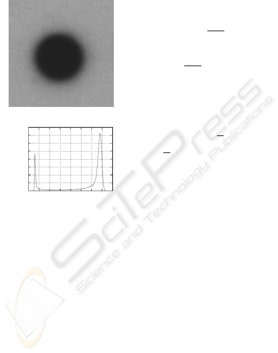
(a) Macroarray dot.
0
200
400
600
800
1000
1200
1400
1600
20 40 60 80 100 120 140 160 180
Count
Intensity
(b) Histogram of 1(a).
Figure 1: Two-dominant intensities image.
decrease should be measured having, as first ending
level, the level where we find the depression between
the two peaks, but, if that could easily be found, there
wouldn’t be needed to proceed, because that is what
we are trying to find. For that reason, the mean in-
tensity level of the image was used as the first ending
level.
Clearly, if the mean is above the point where the
variance starts to decrease, which happens if the least
dominant class (peak) has very little representation in
contrast with the dominant class, the method will not
work, even if there is an important contrast between
classes. Nevertheless, for images where the mean was
below the point of decrease on variation, this solution
finds a fairly good threshold level. So, the variance
was measured, starting from the first intensity level
until the mean intensity, towards the dominant peak,
comparing the result of each step with the previous
one.
Knowing that an image is a 2D grayscale intensity
function with N pixels with graylevels from 1 to L
and the number of pixels of graylevel i is denoted by
f
i
, we can define the mean until level l as:
µ
l
=
l
∑
i=0
i× f
i
∑
l
i=0
f
i
; (1)
and the variance until level l as:
σ
2
l
=
1
∑
l
i=0
f
i
l
∑
i=0
f
i
× (i− µ
l
)
2
. (2)
Assuming that the dominant peak is on the right
side of the histogram (as in image 1(b)), the level
l where σ
2
l
will decrease relatively to σ
2
l−1
, can be
defined as the first occurrence of:
l
∗
= {l | σ
2
l
< σ
2
(l−1)
∧ µ
L
≤ l < L}; (3)
then, the threshold level T, would be:
T = l
∗
−
q
σ
2
L
. (4)
where
q
σ
2
L
is the standard deviation of the whole im-
age.
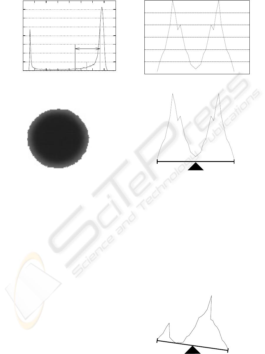
As an example, take the case of the image I in fig-
ure 1(a). The mean intensity of I is µ
L
= 130 and the
standard deviation is σ
L
= 43, with L = 256. Calcu-
lating the variances σ
2
l
with l being the ending lev-
els for calculation of the variance and µ
L
≤ l < L, all
the variances will rise until the gray level is 153 (see
fig. 2), where σ
2
154
< σ
2
153
. Consequently, l
∗
= 154,
and the estimated threshold level is calculated by sub-
tracting the standard deviation of the image from l
∗
.
In this way, we get a threshold value of T = 111 (see
fig. 3). Applying the well known Otsu (Otsu, 1979)
thresholdingmethod, the achievedthreshold level was
of 100. Taking in consideration that in many circum-
stances an acceptable threshold level for this image
could be between the intensities 40 and 140, 111 is
a good threshold level. For the specific case, any
threshold level between 60 and 120, would be a very
good threshold level. When manually thresholding
the same image, the optimum threshold was found as
76. With T = 76, the diffuse area that separates back-
ground and foreground was almost completely elimi-
nated.
As can be seen on figure 2, the variance decreases
when the selected part of the histogram starts to grow
more in height than in spread, meaning that all the
intensity values until l
∗
or higher will be closer to
the mean. On a histogram with both intensity classes
equally expressed, the growth of any of the existing
intensities will decrease the variance. Observing fig-
ure 2, it can be stated that the variance decreases af-
ter the histogram is more or less balanced between
BI-LEVEL IMAGE THRESHOLDING - A Fast Method
71
0
200
400
600
800
1000
1200
1400
1600
20 40 60 80 100 120 140 160 180
Count
Intensity
T
µ
L
l*
σ
L
Figure 2: Calculation of T.
Figure 3: Image 1(a) thresholded with T=110.
the first intensity level and level l
∗
. Also, consider-
ing a histogram with only two intensities, the maxi-
mum variance will be reached when both intensities
are equally expressed. Any increase or decrease to
any of the intensities of the histogram, will result in
the decrement of the variance, because one of the in-
tensities will be dominant.
As stated before, the previous approach would
need images with very specific characteristics and,
that is not allways possible. Although this was not
a good technique for image thresholding it gave us
some ideas on how to find a good thresholding level,
as explained on the next section.
3 WEIGHTING A HISTOGRAM
If a perfect balanced histogram, i.e. a histogram that
has the same distribution of background and fore-
ground, could be placed over a lever, it wouldn’t fall
for any side (see fig. 4). Also, notice that the opti-
mum threshold level would be right in the centre of
the lever.
Looking at figure 5, which represents an unbal-
anced histogram, it can be observed that the lever falls
(a) Balanced Histogram.
(b) Histogram over a lever.
Figure 4: Perfectly balanced histogram.
to the side where the histogram is heavier. The idea
is to try to balance the unbalanced histogram. Once
again, there is the assumption that the image has two
dominant classes (peaks), one representing the fore-
ground and the other representing the background. In
this case, there is no need of one being highly domi-
nant over the other. So, how can an unbalanced his-
togram be balanced? The proposed way of doing it
is to figuratively put the unbalanced histogram over a
lever, as in figure 5, and then start to remove the ex-
cess weight from the heavier side. The next step is to
adjust the base triangle to the new middle position.
I
s
I
m
I
e
Figure 5: Unbalanced Histogram.
BIOSIGNALS 2008 - International Conference on Bio-inspired Systems and Signal Processing
72
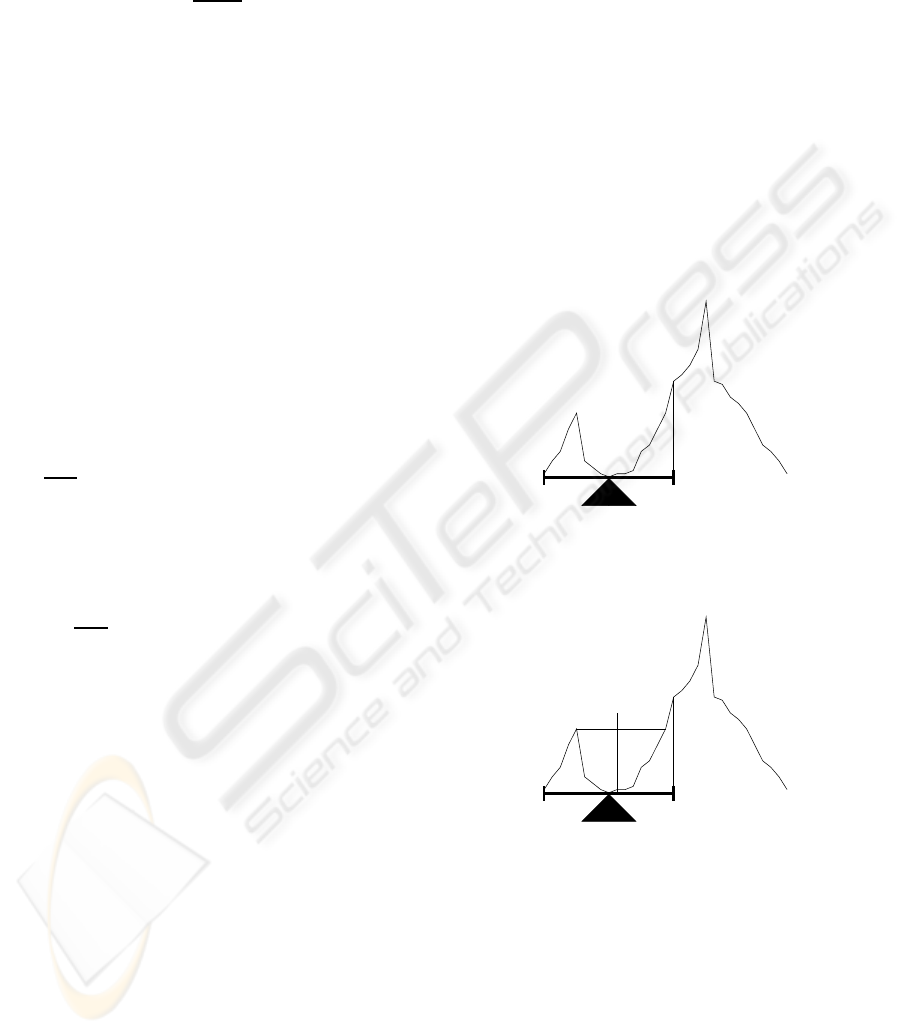
Let I
s
(Intensity Start) be the first graylevel inten-
sity occurrence and I
e
(Intensity End) the last. Now
the position of the base triangle can be defined as:
I
m
=
I
s
+ I
e
2
. (5)
Remembering that an image is a 2D grayscale in-
tensity function with N pixels with graylevels from 1
to L and the number of pixels of graylevel i denoted
by f
i
, we can define the weights of the left and right
sides as:
W
l
=
I
m
∑
i=I
s
f
i
(6)
and
W
r
=
I
e
∑
i=I
m+1
f
i
(7)
so that initially W
l
+ W
r
= N, we can define the
following algorithm:
Algorithm
3.1: GET-THRESHOLD(f, I
s
, I
e
)
I
m
←
I
s
+I
e
2
W
l
←
∑
I
m
i=I
s
f
i
W
r
←
∑
I
e
i=I
m+1
f
i
while W
r
> W
l
do
W
r
← W
r
− f
I
e
I
e
← I
e−1
if
I
s
+I
e
2
< I
m
then
W
l
← W
l
− f
I
m
W
r
← W
r
+ f
I
m
I
m
← I
m
− 1
return (I
m
)
The same algorithm will apply when the dominant
peak is on the left side, only mirrored. Another solu-
tion is to invert the histogram and apply the algorithm
the same way. But for now, it will be assumed that
the most dominant peak (heaviest) is at the right side
of the least dominant one. What happens in this algo-
rithm is that after determining I
s
and I
e
, I
m
, the posi-
tion of the base triangle is calculated (see eq. 5). After
that, two classes are created, W
l
with all the intensi-
ties at the left of I
m
(see eq. 6) and W
r
with all the
intensities at the right of I
m
(see eq. 7). Now, while
the heaviest class (W
r
in this case) weights more than
the lightest, columns are subtracted from the heaviest
peak, starting at the outer side of it. Then, if there is a
need to adjust the position of the base triangle, mov-
ing it to the left, both classes are adjusted accordingly,
W
l
loosing one bar to W
r
. The result of applying the
algorithm on the histogram represented by figure 5
can be seen on figure 6(a).
At the end, I
m
is the position which is in between
the two peaks that may work as a threshold level.
Another estimate for the threshold can be the lowest
value between the highest peak at the left of I
m
and the
highest peak at the right of I
m
or, by other words, the
lowest value between the two peaks. That in not very
hard to find now that we have I
m
. There is another ap-
proach that generally seams to produce better results.
That approach consists of drawing a horizontal line
over the top of the lowest of the two dominant peaks
and determine its intersection with the highest peak.
Then the middle distance between the top of the low-
est dominant peak and that intersection, can be used
as a threshold, as demonstrated by figure 6(b).
I
s
I
m
I
e
(a) Threshold is I
m
.
T
I
m
(b) Threshold is T.
Figure 6: Processed Histogram.
If the image is noisy, the histogram may have
some intensities represented with very low frequency
and usually they will be noticed in the histogram as
tails before the first peak and after the last one. In
this case, using the approach presented by algorithm
3.1 to find a threshold level may fail. For example, if
the least dominant peak has a big tail (see fig. 7), I
s
will be placed very far away from the representative
BI-LEVEL IMAGE THRESHOLDING - A Fast Method
73
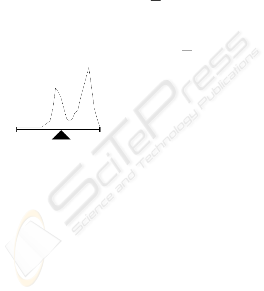
area of the least dominant peak, moving I
m
closer to
the least dominant peak. The approach represented on
figure 6(b) can correct this problem only if the result-
ing I
m
is still between the two peaks. In the case that
it’s the most dominant peak that has the big tail, that
may cause the side that should be the lighter one, to be
the heavier, not allowing to find the right thresholding
level. In order to solve this problem, there have been
found two main approaches. One consists of pass-
ing a parameter to the algorithm that will work as the
least quantity that will be representative and, thus, ac-
counted for the calculation of I
s
and I
e
. The other ap-
proach consists of performing a mean smoothing of
the image. This may eliminate all the intensities that
have almost no representativity.
I
s
I
m
I
e
Figure 7: Big tail at the left of least dominant peak.
4 PROPOSED METHOD
The method presented in the previous section (see
alg. 3.1) has a caveat that makes it unreliable in some
cases. This algorithm will tend to approach I
m
to the
lowest peak, proportionally to the degree of grow-
ing and height of the highest peak. That happens,
of course, because each bar of the highest peak will
correspond to more than one of the lowest peak bars.
This may be a minor problem if the contrast is very
high, but will be noticed in low contrast images with
one of the peaks much higher than the other and with
high accentuation of growth. To solve this problem
it was applied the same reasoning presented in sec-
tion 3. For example, if the right side of the histogram
is the heavier, we will remove bars from the right side
of the histogram. The stop condition for algorithm 3.1
is when the right side gets lighter then the left side. At
this point, the histogram will have its left side heavier
than the right side and, thus, it’s unbalanced. Apply-
ing the same algorithm (mirrored) to the histogram,
the right side will become the heaviest side again, and
so on. The result is that I
s
and I
e
will get closer until
they are equal to I
m
. This approach is represented by
algorithm 4.1.
Algorithm
4.1: GET-THRESHOLD-FINAL(f, I
s
, I
e
)
I
m
←
I
s
+I
e
2
W
l
←
∑
I
m
i=I
s
f
i
W
r
←
∑
I
e
i=I
m+1
f
i
while I
s
6= I
e
do
if W
r
> W
l
then
W
r
← W
r
− f
I
e
I
e
← I
e−1
if
I
s
+I
e
2
< I
m
then
W
l
← W
l
− f
I
m
W
r
← W
r
+ f
I
m
I
m
← I
m−1
else if W
l
≥ W
r
then
W
l
← W
l
+ f
I
s
I
s
← I
s+1
if
I
s
+I
e
2
> I
m
then
W
l
← W
l
+ f
I
m
+1
W
r
← W
r
− f
I
m
+1
I
m
← I
m+1
return (I
m
)
In this way I
m
will tend to move to the lowest area
of the depression in the histogram. With this approach
it won’t matter how fast the highest peak grows be-
cause I
m
will be centred, once again, if I
m
’s initial
position is located in between the two peaks. There
is still the concern of the big tails in the histogram, if
I
m
’s initial position is outside of the depression in the
histogram.
As a final matter, there is the situation when there
is very low contrast between background and fore-
ground. In this case we only have a peak. This will
result on a all or nothing threshold, because the his-
togram will allways be heavier from the same side.
I
s
will still get to be equal to I
e
, but the threshold
level may not be correct. When the histogram has
two peaks, bars will be removed from both sides of
the histogram, so, the solution that was found to this
problem was to place a flag in each of the places
where bars removal occurs. This way we know if it’s
a one or two peaks histogram or if it’s a one peak his-
togram only. In the case of a one peak histogram, a
good approximation for the threshold level may be the
mean of the original histogram minus some constant
or some percentage.
BIOSIGNALS 2008 - International Conference on Bio-inspired Systems and Signal Processing
74
5 RESULTS
For test and comparison of the presented method,
there were used scanned radioactive images of gene
macro arrays. Due to the existence of gradient in
the global image, obviously there could not be used
an optimum global threshold level, so the image was
split in to tiles of spot images (see fig. 8).
Table1, presents the result of applying this al-
gorithm to those images and compares it to the re-
sult of applying various reference methods. Results
are presented in the following order: Manual thresh-
old, Otsu’s, IsoData, Maximum Entropy, Mixture
Modelling and the proposed method’s threshold lev-
els. For the IsoData, Maximum Entropy and Mixture
Modelling threshold methods, it was used ImageJ’s
(Rasband, 2006) implementation.
Table 1: Results of the various thresholding methods.
Spot Man Otsu Iso Max Mix Pro
1 66 80 78 101 113 69
2 60 68 66 89 12 50
3 59 66 64 85 13 55
4 58 83 81 101 118 67
5 80 90 88 107 118 77
6 55 68 66 89 12 54
7 92 92 90 105 116 84
8 57 69 67 94 104 50
9 60 73 71 96 111 59
10 65 78 77 96 112 72
As can be seen in table 1, the proposed method is
the one that, generally, finds lower values for thresh-
olding. As the spot starts to blend with the foreground
(the diffuse area) there will be the depression in the
histogram. That diffuse area increases in intensity
level and in quantity of pixels as it goes from the spot
to the foreground. It is normal, then, that the proposed
method will find the lower threshold levels because,
as stated before, I
m
will tend to move to the lowest
area of the depression of the histogram. Figure 8 is
shown just to present an idea of the criteria that was
used in the manual threshold calculation (the ground
truths).
6 CONCLUSIONS
This is a very fast method that works very well on im-
ages that have a fair amount of background and fore-
ground representation, and with a reasonable contrast
between both, as is the case of scanned radioactive
images of macroarrays. It is a good approach when
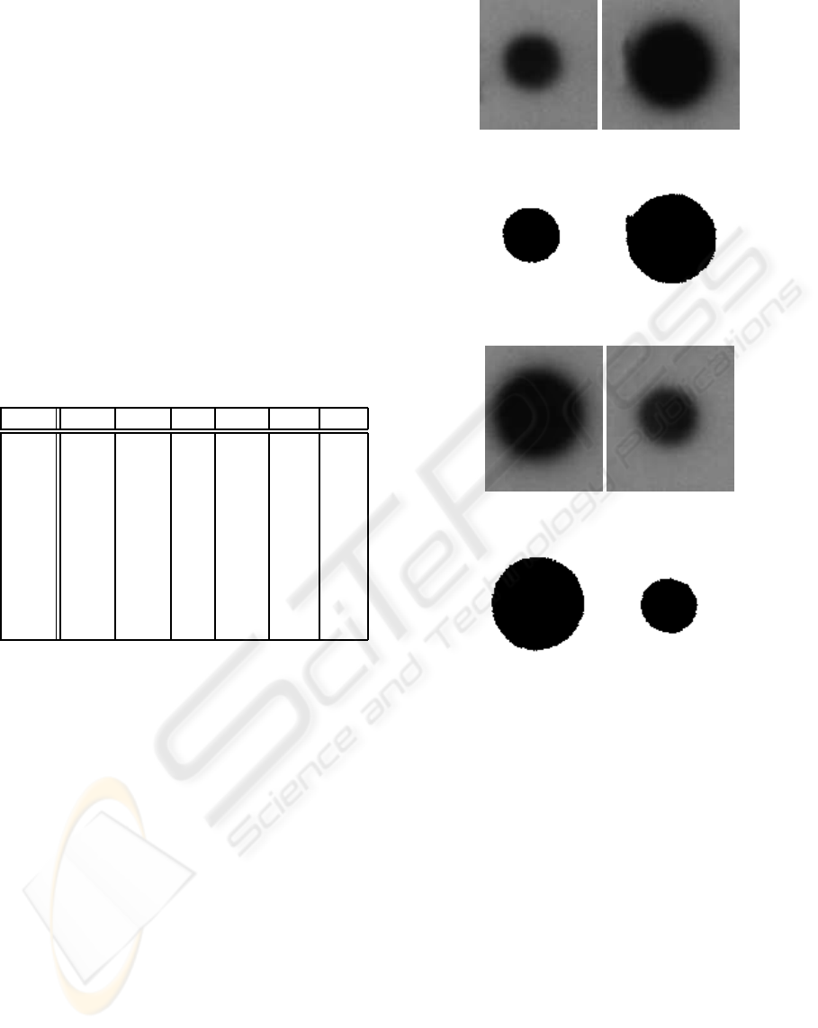
(a) Spot 1. (b) Spot 2.
(c) G. t. of 1 (d) G. t. of 2
(e) Spot 3. (f) Spot 4.
(g) G. t. of 3 (h) G. t. of 4
Figure 8: First four of the tested sample images and their
ground truths.
the objective is to find the spot without the diffuse
area. If the diffuse area is to be included, Otsu or Iso-
data may be better. The presented method is already
being used on a bioinformatics software (Anjos and
Ascenso, 2007) for analysis of gene expression data
of macroarray images.
REFERENCES
Anjos, A., S. H. and Ascenso, R. (2007). Maq - a bioinfor-
matics tool for macroarray analysis. (Internal Report
- ILAB - UAlg).
Diachenko, L., e. a. (1996). Suppression subtractive hy-
bridization: A method for generating differentially
BI-LEVEL IMAGE THRESHOLDING - A Fast Method
75

regulated or tissue-specific cdna probes and libraries.
Proc. Natl. Acad. Sci. USA, 93(12):6025–6030.
Dowsey, Andrew, D. M. and Yang, G.-Z. (2003). The role of
bioinformatics in two-dimensional gel electrophore-
sis. Proteomics, 3(8):1567–1596.
Kamel, M. and Zhao, A. (1993). Extraction of binary
character/graphics images from grayscale document
images. Graphical Model and Image Processing,
55(3):203–217.
Kilian, J. (2001). Simple image analysis by moments.
OpenCV library documentation.
Otsu, N. (1979). A threshold selection method from gray-
level histograms. IEEE Trans. Systems Man Cybernet,
9:62–69.
Rasband, W. (1997-2006). Imagej. U. S. National In-
stitutes of Health, Bethesda, Maryland, USA, page
http://rsb.info.nih.gov/ij/.
Sezgin, M. and Sankur, B. (2004). Survey over image
thresholding techniques and quantitative performance
evaluation. Journal of Electronic Imaging, 13:146–
165.
Sezgin, M. and Tasaltin, R. (2000). A new dichotomisa-
tion technique to multilevel thresholding devoted to
inspection applications. Pattern Recognition Letters,
21:151–161.
Zhang, M. (1999). Large-scale gene expression data anal-
ysis: a new challenge to computational biologists.
Genome Research, 9:681–688.
BIOSIGNALS 2008 - International Conference on Bio-inspired Systems and Signal Processing
76
