FUZZY MRF MODELS WITH MULTIFRACTAL ANALYSIS

FOR MRI BRAIN TISSUE CLASSIFICATION

Liang Geng and Weibei Dou

Department of Electronic Engineering, Tsinghua University, Beijing, P. R. China

Keywords: Brain tissue classification, Fuzzy MRF Model, multifractal analysis.

Abstract: This paper introduces multifractal analysis to the Fuzzy Markov Random Field (MRF) Model, used for

brain tissue classification of Magnetic Resonance Images (MRI). The traditional classifying method using

Fuzzy MRF Model is already able to calculate out the memberships of each voxel, to solve the Partial

Volume Effect (PVE). But its accuracy is relatively low, for its spatial resolution is not high enough.

Therefore the multifractal analysis is brought in to raise the accuracy by providing local information. The

improved method is tests on both simulated data and real images, where results on membership average

errors and position errors are calculated. These results show that the improved method can provide much

higher accuracy.

1 INTRODUCTION

Magnetic Resonance Images (MRI) have been

widely used for brain diagnosis and disorder

detections. Accordingly, segmenting brain images

into different tissues, such as cerebrospinal fluid

(CSF), grey matter (GM) and white matter (WM),

for clinical uses, has become a classical problem.

Many different tissue segmenting methods and

algorithms are proposed these years. Some methods

are using T1 weighted images (Rajapakse et al,

1996), while others use multispectral MR data (Taxt

and Lundervold, 1994). Algorithms can be based on

histogram determination Suzuki and Toriwaki,

1991), or on a priori information on anatomy (Joliot

and Mazoyer, 1993). Mathematical models are used,

from cluster analysis (Simmons et al, 1994) to

Bayesian estimation (Chang et al, 1996). All these

methods assume that each voxel in the images to be

segmented belongs to only one specific tissue.

However, due to the partial volume effect (PVE),

one voxel may contain information from several

different tissues, flawing the segmenting results of

the methods proposed.

To solve the effect of PVE, Markov Random

Field (MRF) Model is applied to tissue classification

(Ruan and Cyril et al, 2000). The a priori

information from an image and the classifying

criteria are combined into energy functions of

MRF’s distribution, and then the voxels with mixed

tissues can be classified by the iterated conditional

mode (ICM). This method achieves a so-called

‘Hard Classifying’, classifying each voxel into one

tissue who contributes the most, and contributions

from other tissues are neglected. Considering that

the neglected information is usually useful, a further

model, the Fuzzy MRF Model, is brought in (Ruan

and Moretti et al, 2001). The Fuzzy MRF Model

takes into account the contextual information, the

statistical information and the anatomical

information of the brain. And ‘Hard Classifying’ is

replaced by ‘Fuzzy Classifying’, providing

‘memberships’ for each voxel, indicating each

voxel’s partial volume degree, in other words,

representing how much these tissues occupy one

voxel respectively.

The fuzzy MRF Model is proved effective on

PVE, but still limitations it has. Experiments show

that this method performs poorly at brinks of brain

images, where grey-level of voxels changes

suddenly, which implies its spatial resolution is not

high enough. Also, this method being noise sensitive,

when it encounters images with high noise, its

accuracy becomes even worse. These limitations can

be attributed to the lack of local properties extracted

from images, so what we need to do is to provide the

Fuzzy MRF abundant local information.

As a new signal processing method, multifractal

analysis is competent for this object. Multifractal is

Geng L. and Dou W. (2008).

FUZZY MRF MODELS WITH MULTIFRACTAL ANALYSIS FOR MRI BRAIN TISSUE CLASSIFICATION.

In Proceedings of the First International Conference on Bio-inspired Systems and Signal Processing, pages 33-39

DOI: 10.5220/0001064400330039

 SciTePress

first studied mathematically (Halsey et al, 1986),

and introduced to image processing by Sarkar and

Katsuragawa (1995). It has derived various methods

for image analysis, and has shown its advantages in

local feature extraction (Liu and Li, 1997). It is also

adapted to MRI brain tissue classifying, to remove

ambiguities in the ‘Hard Classifying’ caused by

intensity overlap, and performed well (Ruan et al,

2000)

Our research aims to raise the spatial resolution

by local information while using fuzzy MRF model.

We propose a combining both fuzzy MRF model

and multifractal analysis together, to achieve a more

accurate ‘Fuzzy Classifying’. In this paper, we

firstly show an overall of the proposed scheme and

two kenel algorithms, fuzzy MRF and multifractal

analysis, then explain how to combine these two

parts in section 2. The validation of this improved

scheme is done both by some experiments and in

comparison with traditional fuzzy MRF method. The

results and discussion are shown in section 3. This

improved algorithm takes the same frame as the

original method, while changes are done

mathematically. Experiments and tests are done on

various images, including real and virtual data with

different amount of added noise.

2 ALGORITHMS

In this section we will introduce the algorithms for

Fuzzy MRF Model along with multifractal analysis.

We will show how the Fuzzy MRF Model works

and how the multifractal information improves its

classifying results.

2.1 A Whole Algorithm for Fuzzy MRF

Model with Multifractal Analysis

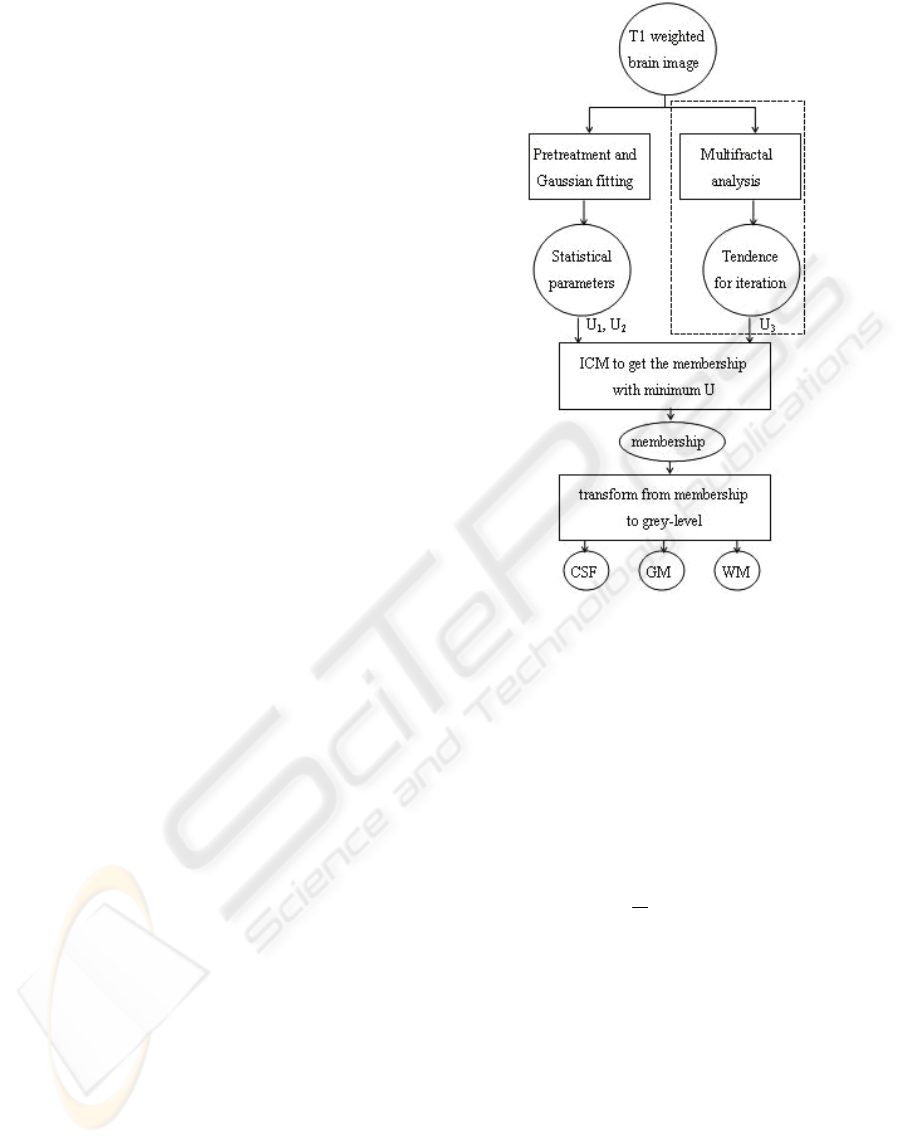
Here we give out the flowchart of the whole

algorithm using Fuzzy MRF Model with multifractal

analysis, as Figure 1.

A parallel treatment, such as a preteatment for

the parameter estimation of Fuzzy MRF Model and

a multifractal analysis for producing a novel

parameter U

to adjust a traditional Fuzzy MRF

Model, is the contribution of this scheme.

The region framed by dashed line rectangle is the

multifractal part added to the original frame. The

other modules form the ICM iteration of Fuzzy MRF

(Ruan and Moretti et al, 2001), and the multifractal

part provides a ‘tendence’ to instruct the iterating

course. We will discuss them in detail in following

subsections.

Figure 1: Flowchart of the whole algorithm.

2.2 Fuzzy MRF Model

The MRF Model is an a priori model, it represents

the spatial correlation of image data. Considering a

random field A with its realization a, in practice we

usually use the joint probability density function of

A on the whole image. Particularly when the

probability density is distributed Gibbsian, the

density function takes form as (1):

( ) exp( ( )),

exp( ( ))

PX x Ux

ZUx

== −

=−

∑

(1)

where U(a) stands for the energy function, and Z the

normalizing constant.

Fuzzy MRF Model applied to image

segmentation, there are two random fields. One is

the membership field A, whose realization is a, the

other is the grey-level field Y, whose realization is y,

which is known a priori. The goal of tissue

classifying is to achieve the maximum joint

probability density distribution of these two random

field:

BIOSIGNALS 2008 - International Conference on Bio-inspired Systems and Signal Processing

|{ ( , ) ( , ), }

result AY A Y

aaPayPxyx=≥∀

(2)

The joint probability can be represented by

conditional probability as:

(, ) () ( | )

AY A Y A

Pay PaPya=

(3)

Comparing (1) and (3), we can get the

probability distribution of Fuzzy MRF of image:

,12

(, ) exp( (, ) ())

Pay UayUa

=− −

(4)

Here U

represents the incompatibility between the

grey-levels and the memberships, and U

represents

the inhomogeneity of memberships themselves.

They can be calculated using statistical parameters,

which are acquired by fitting the grey-level

histogram with several Gaussian functions (Ruan

and Jaggi et al, 2000).

Once the two parts of energy function are

calculated out, we can use the deterministic

relaxation iterated conditional modes (ICM) to find

the optimum realization of membership a, to ensure

the energy function U being minimum, which means

the joint probability in (1) being maximum.

The original algorithm concerns only these two

parts of energy function, and information about the

partial details are not taken into account. So we can

see the shortcome of the original algorithms clearly

by calculating the set-difference between classifying

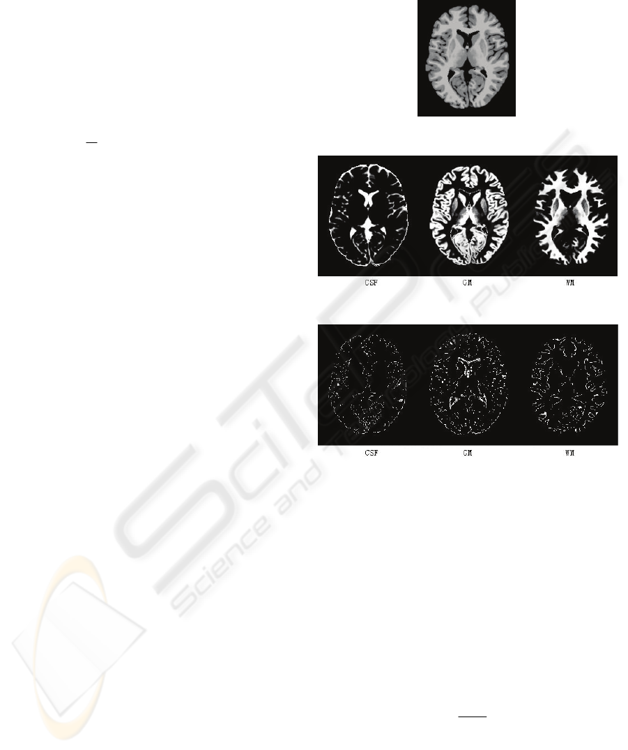
resluts and standard modules. Here we use a noise-

free virtual image of normal brain with no RF. The

original image is shown in Figure 2. Classifying

results are shown in Figure 3 and differences in

Figure 4, as we can see, the spatial differences

mainly locate on the brinks, stings and nicks of the

image, where grey level changes suddenly. If we

could provide the algorithm enough local

information to raise its spatial resolution, the result

should be more accurate.

2.3 Multifractal Analysis

The multifractal analysis is first adopted into ‘Hard

Classification’ by Ruan (Ruan and Bloyet, 2000), to

remove the ambiguity caused by intensity overlap.

The intensity overlap has nothing to do with the

fuzzy model, since in fuzzy circumstances, we need

not to reclassify a mixed voxel into one particular

pure tissue. But the local information provided by

multifractal still helps in raising the spatial

resolution, thus we introduce the multifractal method

to the Fuzzy MRF Model.

Figure 2: The original image named Vn00.

Figure 3: The classifying results of a virtual image.

Figure 4: The spatial difference between classifying

results and standard modules of a virtual image.

2.3.1 Multifractal in Signals

It is well known that fractal is widely used to

process self-similar signals, by providing its global

information of similarity to the ‘fractal dimension’.

But to provide local information, we need the

‘fractal dimension’ to vary from part to part of the

signal. This is multifractal.

Therefore Multifractal dimension is defined

locally by the measurement and length of a

shrinking small region, as (5):

log

lim

log

→

(5)

where

denotes the multifractal dimension, also

called Hölder exponent, b denotes the measurement,

and a the length of the region.

FUZZY MRF MODELS WITH MULTIFRACTAL ANALYSIS FOR MRI BRAIN TISSUE CLASSIFICATION

Each small region has its own Hölder exponent,

and then the whole signal can be considered as the

union of many subsets that combining with each

other. To characterize the local characteristics, we

need another parameter to decompose these small

regions, and group all voxels being in the same kind

of detail into a set. The parameter brought in is

called ‘multifractal spectrum’, defined as

()f

’s definition can be Hausdorff, Legendrea, or

others. We can also define it particularly.

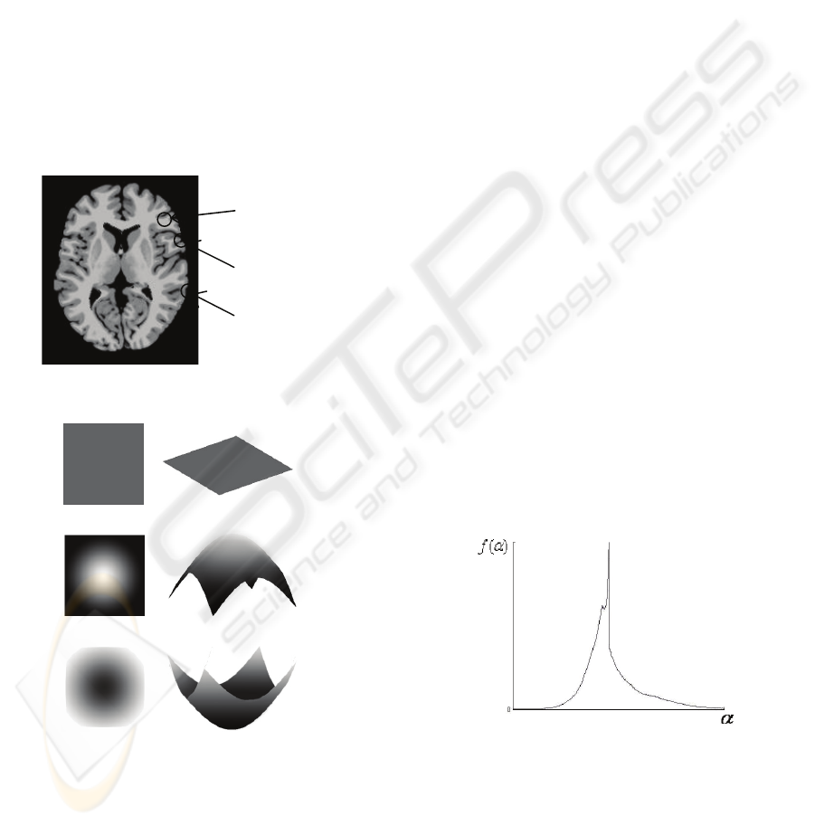
2.3.2 Multifractal in Brain Images

To describe the local details of brain images, first we

need to abstract these details into several simple

models. Observe the images, we can find out three

kinds of details shown in Figure 5.

Figure 5: The details of brain image.

(a) plain detail

(b) hill detail

Figure 6: The models of details. The intensity model is on

the left, while grey-level model is on the right.

Grey levels of voxels in plain region has little

difference from the central voxel, most of the small

regions are proved to be plain. Hill region has

several voxels much lighter in the centre, and valley

region has a much darker centre. The models can be

illustrated as Figure 6.

After defined the three detail models, the Hölder

exponent

is ready to be calculated out for each

model. From the equation (5) we could know that

is defined to be a limit process. Because the image is

composed by discrete voxels, the values of length a

must also be discrete, thus the limit process is

discrete: first a takes the radius of the small region R

as its value, then each time a minus 1 until a

becomes 0. The corresponding value of b is the sum

of grey level of voxels in a diminishing spherical

small region whose radius is a. Both a and b gotten,

the Hölder exponent

can be gotten in succession.

Since we only care about the relative size of the

Hölder exponent

, the values themselves make no

sense to us; we can also use some approximate

method, such as linear fitting, instead of the

complicate limit process.

At last, we can get the relative size of the Hölder

exponent

in different details: for hill,

relatively smaller, and for valley,

is relatively

bigger, while for plain, it’s in the middle.

To decompose image details and group the

voxels into three sets,

()f

needs to be generated

from

. And for concision, we define

()f

’s

histogram, that means:

() ((),)

δα α

∈

∑

(6)

where I represents the whole image,

()k

is the

Hölder exponent at voxel k,

((), )

αα

Kronecker Function, which takes the value 1 while

()

, and 0 while

()

≠

Figure 7: Multifractal spectrum of MR brain image.

Then we get the histogram as spectrum, shown in

Figure 7. A correctly collected MR Brain image

must has a multiractal spectrum in this shape,

because most voxels are in plain regions, which

makes the high peak in the middle. Therefore we

need only to find the position of the peak, denoted as

plain

hill

valley

BIOSIGNALS 2008 - International Conference on Bio-inspired Systems and Signal Processing

, representing the corresponding voxels being in

plain detail, and voxels with an

smaller than

are in hill regions, others are in valley regions.

2.4 Multifractal Applied to Fuzzy MRF

Using multifractal, we can label every voxel the

detail type it belongs to, and the rest to be done is to

combine the multifractal and Fuzzy MRF together,

by influencing the ICM iterating process with these

detail labels.

We consider translating the labels into some sort

of ‘tendence’. If a voxel is labelled ‘hill’, that means

it’s brighter than its neighbours, then it should have

a tendence to be classified into a brighter tissue. If

the voxel is labelled ‘valley’, on contrary, it should

have a tendence to be classified into a darker tissue.

If the voxel is labelled ‘plain’, its brightness is

almost the same as its neighbours’, so it should have

no tendence.

Then the main problem is how to translate the

detail labels into ‘tendences’. Here we propose the

energy function U

, to change the value of U,

therefore to impose the ‘tendence’ to the iterating

process. From to gradient label (denoted by D), then

to U

, can be defined as equation (7):

1()

0(),

1()

0 , 0,

hill

hill valley

valley

current

fractal current fractal

current

hill

Dplain

valley

UD aa

αα

ααα

αα

ββ

⎧

⎪

=≤≤

⎨

⎪

−>

⎩

−>

⎧

⎪

=⋅ ⋅ = >

⎨

⎪

⎩

(7)

For equation (7),

hill

and

valley

are thresholds

generated from the spectrum

()f

shown in Figure

7, e.g,

max( | ( ) ( ) / 2 & )

hill

αα α αα

=<<

and

min( | ( ) ( ) / 2 & )

valley

αα α αα

=<>

And

fractal

is a positive weight coefficient for U

whose value depends on how much you want the

multifractal part to affect the whole system.

Using (7), the detail ‘hill’ can make U with

brighter membership a smaller, and U with darker

membership a bigger. For the detail ‘valley’, the

performance is on the contrary. Thus multifractal

can be applied to the algorithm frame shown in

Figure 1.

3 EXPERIMENTS AND RESULTS

3.1 Experiment Materials

Experiments are done on 9 data sets to test the

improved algorithm. These 9 sets of data includes

various conditions, such as virtual data and real

images, data with different noise levels and RF

levels, data of normal brains and brains with defect.

We name each image the way as following. The 1

letter indicates its source in V (virtual) and R (real).

The 2

letter indicates the defect of the brain, in n

(normal), s (multiple sclerosis) and t (tumour). The

number indicates its noise level in percent. And

the 2

number indicates whether RF is added, in 1 if

added or 0 if not.

The information of the 9 sets of data is listed in

Table 1.

Table 1: Information of data sets used for tests.

Name Source Defect Noise RF

Vn00 virtual normal 0% 0%

Vn30 virtual normal 3% 0%

Vn50 virtual normal 5% 0%

Vn70 virtual normal 7% 0%

Vn01 virtual normal 0% 20%

Vn71 virtual normal 7% 20%

Vs00 virtual

multiple

sclerosis

0% 0%

Rn real normal

Rt real tumour

To quantify the tests of accuracy, we mainly use

the virtual data and their standard modules. The

virtual data is from Montréal Neurological Institute,

McGill University, McConnell Brain Imaging

Centre (Website: http://www.bic.mni.mcgill.ca/

brainweb/

3.2 Evaluating Method

The classifying results of virtual images are

evaluated in two ways. The 1

way is the position

error e

, which is the number of voxels classified

differently from the standard module. The position

error is defined as equation (8).

FUZZY MRF MODELS WITH MULTIFRACTAL ANALYSIS FOR MRI BRAIN TISSUE CLASSIFICATION

(,,) (,,)

(, , )

(, , ) (, , )

(,)

p result i jk std i jk

ijk I

result i j k std i j k

eaa

∈

⎧

⎨

≠

⎩

∑

(8)

And the 2

way is the membership average error

, which indicates the average error of

memberships from the whole images. The

membership average error is defined as equation (9),

where N(I) represents the number of voxels.

(, , ) (, , )

(, , )

()

result i j k std i j k

ijk I

∈

−

∑

(9)

3.3 Result and Discussion

The position error of each image data using each

algorithm is listed in Table 2, the membership

average errors are listed in Table 3.

Both Table 2 and Table 3 show that the

algorithm with multifractal has lower errors, in other

words, higher accuracy than the original one. (In

spite of some exceptions caused by noise and RF,

such as GMs of Vn50 and Vn01 in Table 2, the

flaws can be compensated by better results on the

other tissues. )

Table 2: Position errors of two algorithms.

(number of voxels)

Data

Multi-

fractal

CSF GM WM

without 68232 105738 55071

Vn00

with 66398 98904 54122

without 114829 140443 139721

Vn30

with 115507 134358 139774

without 188361 193855 223821

Vn50

with 183362 194035 222067

without 228503 238072 281032

Vn70

with 228273 230507 278875

without 165458 255996 195482

Vn01

with 166628 256531 190323

without 232630 256904 306778

Vn71

with 232336 250765 302827

without 72145 124560 72968

Vs00

with 72170 119322 69315

Table 3: Membership average errors of two algorithms.

Data

Multi-

fractal

CSF GM WM

without 1.6322 3.3685 1.3824

Vn00

with 1.5104 3.1752 1.3422

without 2.1395 4.9949 2.7958

Vn30

with 2.0264 4.8018 2.7688

without 2.9763 7.4779 4.6330

Vn50

with 2.8443 7.2597 4.5960

without 4.3948 9.4826 5.9437

Vn70

with 3.5422 9.1410 5.9312

without 2.3392 6.2700 3.9262

Vn01

with 2.2365 6.1273 3.8102

without 3.8495 10.526 7.0626

Vn71

with 3.6663 10.136 7.0032

without 1.6992 3.4159 1.4649

Vs00

with 1.6233 3.2771 1.4197

Because of the effect of other tissues such as

muscles and bones, the errors are still not very low,

but we could observe just the voxels at brinks, which

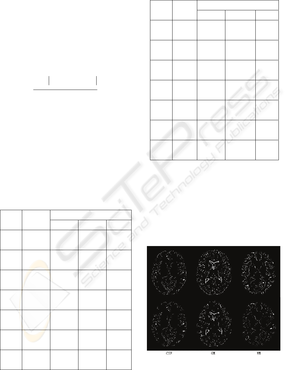
we care about. Comparing the result images, we find

that the voxels improved are mainly what we wanted

to improve. Compare to the results from original

method, the results of multifractal method have

much less error voxels at the brinks of images. One

comparison of position error using Vn00, the same

data as Figure 2, is shown in Figure 8.

Figure 8: Position error of original algorithm (above) and

improved algorithm with multifractal (below).

BIOSIGNALS 2008 - International Conference on Bio-inspired Systems and Signal Processing

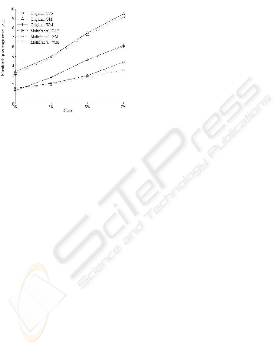
Figure 9: Membership average error of original algorithm

(real line) and improved algorithm with multifractal

(dotted line).

Another improvement is the better robustness on

noise. We chart the average errors of Vn00 to Vn07

in Table 2, the curves are shown in Figure 9.

The higher the noise level becomes, the greater

the accuracy improves. The improved method with

multifractal is improved less sensitive to noise, and

can be used to contain the deterioration caused by

high noise.

Results of real image Rn and Rt have been

compared to some manual segmenting results, and

they match each other. The improved method can be

well used for real applications.

4 CONCLUSIONS

An improvement from multifractal analysis has been

done to the traditional tissue classifying algorithm

using Fuzzy MRF Model. The original mathematical

models and fuzzy features are reserved, when spatial

resolution is increased, thus accuracy is improved. In

numbers of tests on various sorts of data, the

improved method shows its advantage on accuracy

to the original method. Also an entire algorithm

using the improved method is proposed and tested,

doing well in real applications.

ACKNOWLEDGEMENTS

This work is supported by Project NSFC-60372023,

the National Natural Science Foundation of China.

We would like to give special thanks to Su Ruan,

Jean-Marc Constans and Lab of GREYC-

ENSICAEN CNRS UMR 6072 of France for

providing us their research experience and

experimental code.

REFERENCES

Rajapakse, J.C., Giedd, J.N., DeCarli, C., Snell, J.W.,

McLaughlin, A., Vauss, Y.C., Krain, A.L., Hamburger,

S., Rapoport, J.L., 1996. A technique for single

channel MR brain tissue segmentation: application to a

pediatric sample. Magn Res Imag, 14, 1053~1065.

Taxt, T., Lundervold, A., 1994. Multispectral analysis of

the brain using magnetic resonance imaging. IEEE

Trans Med Imag, 13, 470~481.

Suzuki, H., Toriwaki, J., 1991. Automatic segmentation of

head MRI images by knowledge guided thresholding.

Comput Med Imag Graph, 15, 233~240.

Joliot, M., Mazoyer, B., 1993. Three-dimensional

segmentation and interpolation of magnetic resonance

brain images. IEEE Trans Med Imag, 12, 269~277.

Simmons, A., Arridge, S.R., Barker, G.J., Cluckie, A.J.,

Tofts, P.S., 1994. Improvement to the quality of MRI

cluster analysis. Magn Res Imag, 12, 1191~1204.

Chang, M.M., Sezan, M.I., Tekalp, A.M., Berg, M.J., 1996.

Bayesian segmentation of multislice brain magnetic

resonance imaging using threedimensional Gibbsian

Priors. Optical Engineering, 35, 3206~3221.

Ruan, S., Jaggi, C., Xue, J., Fadili, J., Bloyet, D., 2000.

Brain Tissue Classification of Magnetic Resonance

Images Using Partial Volume Modeling. IEEE Trans

Med Imag, 19, 1179~1187.

Ruan, S., Moretti, B., Fadili,J., and Bloyet, D., 2001.

Segmentation of Magnetic Resonance Images using

Fuzzy Markov Random Fields. IEEE, 3, 1051~1054.

Halsey, T.C., Jensen, M.H., Kadanoff, L.P., Procaccia, I.,

Shraiman, B.I., 1986. Fractal measures and their

singularities, the characterization of strange sets. Phys.

Rev., 33, 1141–1151.

Sarkar, N., Katsuragawa, S., 1995. Multifractal and

generalized dimension of gray-tone digital images.

Signal Processing, 42, 181~190.

Liu, Y., Li, Y., 1997. New approaches of multifractal

image analysis. IEEE-ICICS’ 1997, 2, 970~974.

Ruan, S., Bloyet, D., 2000. MRF Models and Multifractal

Analysis for MRI Segmentation. IEEE-ICSP’2000, 2,

1259~1262.

FUZZY MRF MODELS WITH MULTIFRACTAL ANALYSIS FOR MRI BRAIN TISSUE CLASSIFICATION