
FAST AND ROBUST MID-SAGITTAL PLANE LOCATION
IN 3D MR IMAGES OF THE BRAIN
Felipe P. G. Bergo, Guilherme C. S. Ruppert, Luiz F. Pinto and Alexandre X. Falc˜ao
LIV, Institute of Computing, Unicamp, C.P. 6176, Campinas, SP, 13083-970, Brazil
Keywords:
Mid-sagittal plane extraction, medical image analysis, medical image alignment, brain image segmentation.
Abstract:
Extraction of the mid-sagittal plane (MSP) is an important step for brain image registration and asymmetry
analysis. We present a fast MSP extraction method for 3D MR images, which is based on automatic segmen-
tation of the brain and on heuristic maximization of cerebro-spinal fluid within the MSP. The method is shown
to be robust to severe anatomical asymmetries between the hemispheres, caused by surgical procedures and
lesions. The experiments used 64 MR images (36 pathological, 20 healthy, 8 synthetic) and the method found
an acceptable approximation of the MSP in all images with a mean time of 60.0 seconds per image.
1 INTRODUCTION
The human brain is not perfectly symmetric (David-
son and Hugdahl, 1996; Crow, 1993; Geschwind
and Levitsky, 1968). However, for the purpose
of analysis, it is paramount to define and distin-
guish a standard of asymmetry, considered as normal
for any given measurement, from abnormal asym-
metry, which may be related to neurological dis-
eases, cerebral malformations, surgical procedures
or trauma. Several works sustain this claim. For
example, accentuated asymmetries between left and
right hippocampi have been found in patients with
Schizophrenia (Wang et al., 2001; Csernansky et al.,
1998; Styner and Gerig, 2000; Mackay et al., 2003;
Highley et al., 2003; Barrick et al., 2005), Epilepsy
(Hogan et al., 2000; Wu et al., 2005) and Alzheimer
Disease (Csernansky et al., 2000; Liu et al., 2007).
The brain can be divided in two hemispheres, and
the structures of one side should have their counter-
part in the other side with similar shapes and approxi-
mate locations (Davidson and Hugdahl, 1996). These
hemispheres have their boundaries limited by the lon-
gitudinal (median) fissure, being the corpus callosum
their only interconnection.
The ideal separation surface between the hemis-
feres is not perfectly planar, but the mid-sagittal plane
(MSP) can be used as a reference for asymmetry anal-
ysis, without significant loss in the relative compar-
ison between normal and abnormal subjects. The
MSP location is also important for image registration.
Some works have used this operation as a first step for
intra-subject registration, as it reduces the number of
degrees of freedom (Ardekani et al., 1997; Kapouleas
et al., 1991), and to bring different images into a same
coordinate system (Liu et al., 2001), such as in the Ta-
lairach (Talairach and Tournoux, 1988) model.
However, there is no exact definition of the MSP
and its determination by manual delineation is sen-
sitive to different experts. Given that, a reasonable
approach for evaluation seems to be visual inspection
with error quantification, when we increase the asym-
metry artificially and/or linearly transform the image.
The longitudinal fissure forms a gap between the
hemispheres filled with cerebro-spinal fluid (CSF).
We define the MSP as a large intersection between
a plane and an envelope of the brain (a binary vol-
ume whose surface approximates the convex hull of
the brain) that maximizes the amount of CSF. This
definition leads to an automatic, robust and fast algo-
rithm for MSP extraction.
The paper is organized as follows. In Section 2,
we review existing works on automatic location of the
mid-sagittal plane. In section 3, we present the pro-
posed method. In section 4, we show experimental
results and validation with simulated and real MR-T1
images. Section 5 states our conclusions.
2 RELATED WORKS
MSP extraction methods can be divided in two
groups: (i) methods that define the MSP as a
92
P. G. Bergo F., C. S. Ruppert G., F. Pinto L. and X. Falcaõ A. (2008).
FAST AND ROBUST MID-SAGITTAL PLANE LOCATION IN 3D MR IMAGES OF THE BRAIN.
In Proceedings of the First International Conference on Bio-inspired Systems and Signal Processing, pages 92-99
DOI: 10.5220/0001066100920099
Copyright
c
SciTePress

plane that maximizes a symmetry measure, extracted
from both sides of the image (Junck et al., 1990;
Minoshima et al., 1992; Sun and Sherrah, 1997;
Ardekani et al., 1997; Smith and Jenkinson, 1999; Liu
et al., 2001; Prima et al., 2002; Tuzikov et al., 2003;
Teverovskiy and Liu, 2006), and (ii) methods that de-
tect the longitudinal fissure to estimate the location of
the MSP (Brummer, 1991; Guillemaud et al., 1996;
Hu and Nowinski, 2003; Volkau et al., 2006). Table
1 summarizes these works, and extensive reviews can
be found in (Hu and Nowinski, 2003), (Volkau et al.,
2006), (Prima et al., 2002) and (Liu et al., 2001).
Methods in the first group address the problem by
exploiting the hough symmetry of the brain. Basi-
cally, they consist in defining a symmetry measure
and searching for the plane that maximizes this score.
Methods in the second group find the MSP by detect-
ing the longitudinal fissure. Even though the longitu-
dinal fissure is not visible in some modalities, such
as PET and SPECT, it clearly appears in MR im-
ages. Particularly, we prefer these methods because
patients may have very asymmetric brains and we be-
lieve this would affect the symmetry measure and,
consequently, the MSP detection.
The aforementioned approaches based on longitu-
dinal fissure detection present some limitations that
we are circumventing in the proposed method. In
(Guillemaud et al., 1996), the MSP is found by using
snakes and orthogonal regression for a set of points
manually placed on each slice along the longitudi-
nal fissure, thus requiring human intervention. Other
method (Brummer, 1991) uses the Hough Trans-
form to automatically detect straight lines on each
slice (Brummer, 1991), but it does not perform well
on pathological images. The method in (Hu and
Nowinski, 2003) assumes local symmetry near the
plane, which is not verified in many cases (see Fig-
ures 2, 5 and 8). Volkau et al. (Volkau et al., 2006)
propose a method based on the Kullback and Leibler’s
measure for intensity histograms in consecutive can-
didate planes (image slices). The method presents ex-
cellent results under a few limitations related to ro-
tation, search region of the plane, and pathological
images.
3 METHODS
Our method is based on detection of the longitudinal
fissure, which is clearly visible in MR images. Un-
like some previous works, our approach is fully 3D,
automatic, and applicable to images of patients with
severe asymmetries.
We assume that the mid-sagittal plane is a plane
that contains a maximal area of cerebro-spinal fluid
(CSF), excluding ventricles and lesions. In MR T1
images, CSF appears as low intensity pixels, so the
task is reduced to the search of a sagittal plane that
minimizes the mean voxelintensity within a mask that
disregards voxels from large CSF structures and vox-
els outside the brain.
The method is divided in two stages. First, we
automatically segment the brain and morphologically
remove thick CSF structures from it, obtaining a brain
mask. The second stage is the location of the plane it-
self, searching for a plane that minimizes the mean
voxel intensity within its intersection with the brain
mask. Our method uses some morphological opera-
tions whose structuring elements are defined based on
the image resolution. To keep the method description
independent of image resolution, we use the notation
S
r
to denote a spherical structuring element of radius
r mm.
3.1 Segmentation Stage
We use the tree pruning approach to segment the
brain. Tree pruning (Falc˜ao et al., 2004a; Miranda
et al., 2006) is a segmentation method based on the
Image Foresting Transform (Falc˜ao et al., 2004b),
which is a general tool for the design of fast im-
age processing operators based on connectivity. In
tree pruning, we interpret the image as a graph, and
compute an optimum path forest from a set of seed
voxels inside the object. A gradient-like image with
high pixel intensities along object borders must be
computed to provide the edge weights of the implicit
graph. A combinatorial property of the forest is ex-
ploited to prune tree paths at the object’s border, lim-
iting the forest to the object being segmented.
To segment the brain (white matter (WM), gray
matter (GM) and ventricles), we compute a suitable
gradient image, a set of seed voxels inside the brain
and apply the tree pruning algorithm. A more detailed
description of this procedure is given in (Bergo et al.,
2007). Note that any other brain segmentation method
could be used for this purpose.
Gradient Computation. MR-T1 images of the
brain contain two large clusters: the first with air,
bone and CSF (lower intensities), and the second,
with higher intensities, consists of GM, WM, skin, fat
and muscles. Otsu’s optimal threshold (Otsu, 1979)
can separate these clusters (Figs. 1a and 1b), such
that the GM/CSF border becomes part of the border
between them. To enhance the GM/CSF border, we
multiply each voxel intensity I(p) by a weight w(p)
as follows:
FAST AND ROBUST MID-SAGITTAL PLANE LOCATION IN 3D MR IMAGES OF THE BRAIN
93
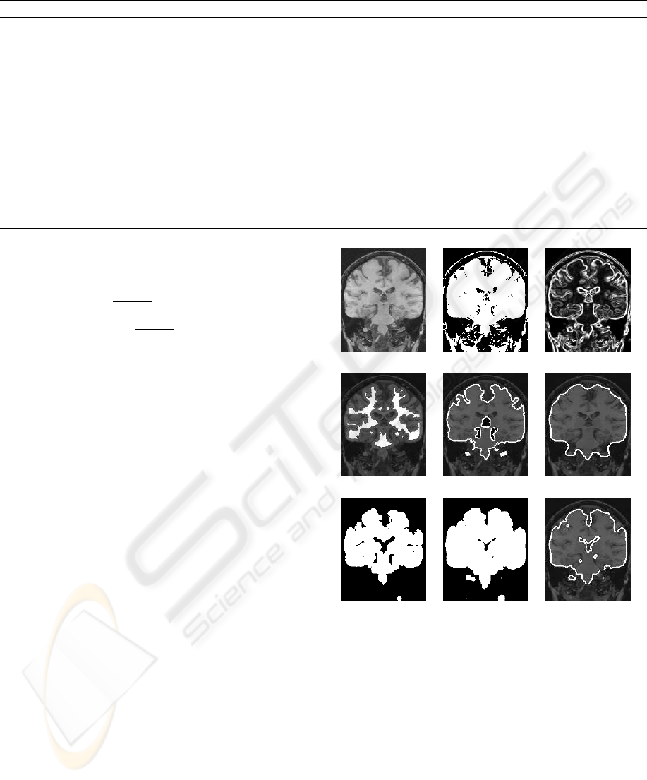
Table 1: Summary of existing MSP methods.
Method Based on 2D/3D Application Measure
(Brummer, 1991) fissure 2D MR Edge Hough Transform
(Guillemaud et al., 1996) fissure 2D MR Active contours
(Hu and Nowinski, 2003) fissure 2D MR, CT Local symmetry of fissure
(Volkau et al., 2006) fissure 3D MR, CT Kullback-Leibler’s measure
(Junck et al., 1990) symmetry 2D PET, SPECT Intensity cross correlation
(Minoshima et al., 1992) symmetry 3D PET Stochastic sign change
(Ardekani et al., 1997) symmetry 3D MR, PET Intensity cross correlation
(Sun and Sherrah, 1997) symmetry 3D MR, CT Extended Gaussian image
(Smith and Jenkinson, 1999) symmetry 3D MR, CT, PET, SPECT Ratio of intensity profiles
(Liu et al., 2001) symmetry 2D MR, CT Edge cross correlation
(Prima et al., 2002) symmetry 3D MR, CT, PET, SPECT Intensity cross correlation
(Tuzikov et al., 2003) symmetry 3D MR, CT, SPECT Intensity cross correlation
(Teverovskiy and Liu, 2006) symmetry 3D MR Edge cross correlation
w(p) =
0 I(p) ≤ m
1
2
I(p)−m
1
m
2
−m
1
2
m
1
< I(p) ≤ τ
1− 2
I(p)−m
2
m
2
−m
1
2
τ < I(p) ≤ m
2
2 I(p) > m
2
(1)
where τ is the Otsu’s threshold, and m
1
and m
2
are the
mean intensities of each cluster. We compute a 3D
gradient at each voxel as the sum of its projections
along 26 directions around the voxel, and then use its
magnitude for tree pruning (Figure 1c).
Seed Selection. The brighter cluster contains many
voxels outside the brain (Figure 1b). To obtain a set of
seeds inside the brain, we apply a morphological ero-
sion by S
5
on the binary image of the brighter clus-
ter. This operation disconnects the brain from adja-
cent structures. We then select the largest connected
component as the seed set (Figure 1d).
Morphological Closing. The brain object obtained
by tree pruning (Figure 1e) might not include the en-
tire longitudinal fissure, especially when the fissure is
too thick. To ensure its inclusion, we apply a mor-
phological closing by S
20
to the binary brain image
(Figure 1f).
Thick CSF Structure Removal. The last step of
this phase is the removalof thick CSF structures (such
as the ventricles, lesions and post-surgery cavities)
from the brain object, to avoid the MSP from snap-
ping to a dark structure other than the longitudinal
fissure. We achieve this with a sequence of mor-
phological operations: we start from a binary image
obtained by thresholding at Otsu’s optimal threshold
(Figure 1b). We apply a morphological opening by
(a) (b) (c)
(d) (e) (f)
(g) (h) (i)
Figure 1: Sample slice of the intermediary steps in stage
1: (a) original coronal MR slice; (b) binary cluster mask
obtained by thresholding; (c) gradient-like image used for
tree pruning; (d) seed set used for tree pruning (white); (e)
border of the brain object obtained by tree pruning (white);
(f) border of the brain object after morphological closing;
(g) CSF mask after opening; (h) CSF mask after dilation;
(h) brain mask (intersection of (f) and (h)).
S
5
to connect the thick (> 5 mm) CSF structures
(Figure 1g), and then dilate the result by S
2
to include
a thin (2 mm) wall of the CSF structures (Figure 1h).
This dilation ensures the reinclusion of the longitudi-
nal fissure, in case it is removed by the opening. The
binary intersection of this image with the brain ob-
BIOSIGNALS 2008 - International Conference on Bio-inspired Systems and Signal Processing
94
ject is then used as brain mask (Figure 1i) by the next
stage of our method. Only voxels within this mask are
considered by stage 2. Figures 2a and 2b show how
the computed brain mask excludes the large cavity in
a post-surgery image, and figures 2c and 2d show how
the mask excludes most of the ventricles in patients
with large ventricles.
3.2 Plane Location Stage
To obtain the CSF score of a plane, we compute the
mean voxel intensity in the intersection between the
plane and the brain mask (Figures 3a and 3b). The
lower the score, the more likely the plane is to contain
more CSF than white matter and gray matter. The
plane with a sufficiently large brain mask intersection
and minimal score is the most likely to be the mid-
sagittal plane.
To find a starting candidate plane, we compute the
score of all sagittal planes in 1 mm intervals (which
leads to 140–180 planes in usual MR datasets), and
select the plane with minimum score. Planes with in-
tersection area lower than 10 000 mm
2
are not consid-
ered to avoid selecting planes tangent to the surface
of the brain. Planes with small intersection areas may
lead to low scores due to alignment with sulci and also
due to partial volume effect between gray matter and
CSF (Figures 3c and 3d).
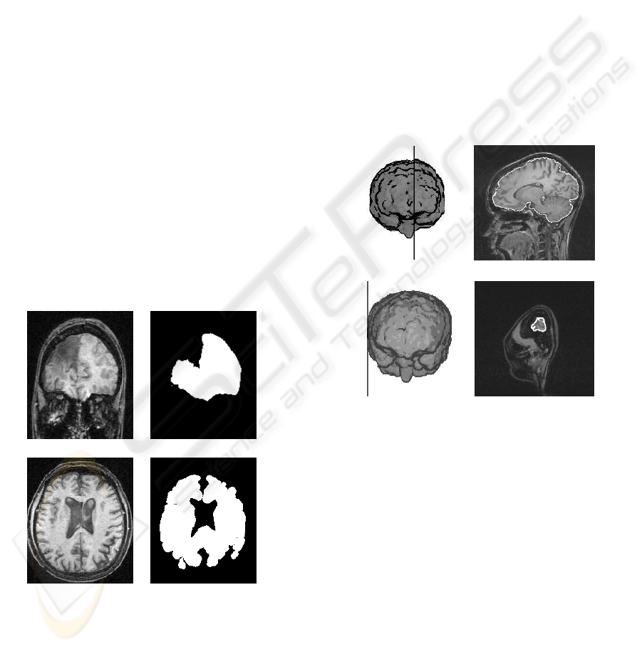
(a) (b)
(c) (d)
Figure 2: Examples of thick CSF structure removal: (a)
coronal MR slice of a patient with post-surgical cavity; (b)
brain mask of (a); (c) axial MR slice of a patient with large
ventricles; (d) brain mask of (c).
Once the best candidate plane is found, we com-
pute the CSF score for small transformations of the
plane by a set of rotations and translations. If none
of the transformations lead to a plane with lower CSF
score, the current plane is the mid-sagittal plane and
the algorithm stops. Otherwise, the transformed plane
with lower CSF score is considered the current candi-
date, and the algorithm is repeated. The algorithm
is finite, since each iteration reduces the CSF score,
and the CSF score is limited by the voxel intensity
domain.
We use a set of 42 candidate transforms at each
iteration: translations on both directions of the X, Y
and Z axes by 10 mm, 5 mm and 1 mm (18 transla-
tions) and rotations on both directions around the X,
Y and Z axes by 10
o
, 5
o
, 1
o
and 0.5
o
(24 rotations).
All rotations are about the central point of the initial
candidate plane. There is no point in attempting ro-
tations by less than 0.5
o
, as this is close to the limit
where planes fall over the same voxels for typical MR
datasets, as discussed in Section 4.1.
(a) (b)
(c) (d)
Figure 3: Plane intersection: (a–b) sample plane, brain
mask and their intersection (white outline). (c–d) exam-
ple of a plane tangent to the brain’s surface and its small
intersection area with the brain mask (delineated in white),
overlaid on the original MR image.
4 EVALUATION AND
DISCUSSION
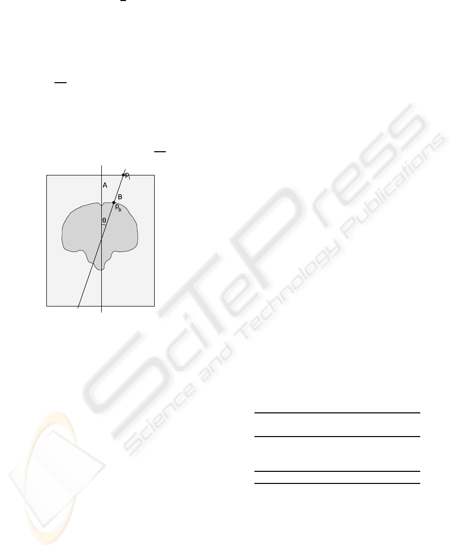
4.1 Error Measurement
The discretization of R
3
makes planes that differ by
small angles to fall over the same voxels. Consider
two planes A and B that differ by an angle Θ (Fig-
ure 4). The minimum angle that makes A and B differ
by at least 1 voxel at a distance r from the rotation
center is given by Equation 2.
FAST AND ROBUST MID-SAGITTAL PLANE LOCATION IN 3D MR IMAGES OF THE BRAIN
95
Θ = arctan
1
r
(2)
An MR dataset with 1 mm
3
voxels has a typi-
cal maximum dimension of 256 mm. For rotations
about the center of the volume, the minimum angle
that makes planes A and B differ by at least one voxel
within the volume (point p
i
in Figure 4) is approxi-
mately arctan
1
128
= 0.45
o
. For most MSP applica-
tions, we are only concerned about plane differences
within the brain. The largest length within the brain is
usually longitudinal, reaching up to 200 mm in adult
brains. The minimum angle that makes planes A and
B differ by at least one voxel within the brain (point
p
b
in Figure 4) is approximately arctan
1
100
= 0.57
o
.
Figure 4: Error measurement in discrete space: points and
angles.
Therefore, we can consider errors around 1
o
ex-
cellent and equivalent results.
4.2 Experiments
We evaluated the method on 64 MR datasets di-
vided in 3 groups: A control group with 20 datasets
from subjects with no anomalies, a surgery group
with 36 datasets from patients with significant struc-
tural variations due to brain surgery, and a phantom
group with 8 synthetic datasets with varying levels
of noise and inomogeneity, taken from the BrainWeb
project (Collins et al., 1998).
All datasets in the control group and most datasets
in the surgery group were acquired with a voxel size
of 0.98 × 0.98 × 1.00 mm
3
. Some images in the
surgery group were acquired with a voxel size of
0.98 × 0.98 × 1.50 mm
3
. The images in the phantom
group were generated with an isotropic voxel size of
1.00 mm
3
. All volumes in the control and surgery
groups were interpolated to an isotropic voxel size of
0.98 mm
3
before applying the method.
For each of the 64 datasets, we generated 10 vari-
ations (tilted datasets) by applying 10 random trans-
forms composed of translations and rotations of up to
12 mm and 12
o
in all axes. The method was applied
to the 704 datasets (64 untilted, 640 tilted), and visual
inspection showedthat the method correctly found ac-
ceptable approximations of the MSP in all of them.
Figure 5 shows sample slices of some datasets and
the computed MSPs.
For each tilted dataset, we applied the inverse
transform to the computed mid-sagittal plane to
project it on its respective untilted dataset space.
Thus, for each untilted dataset we obtained 11 planes
which should be similar. We measured the angle be-
tween all
11
2
= 55 distinct plane pairs. Table 2 shows
the mean and standard deviation (σ) of these angles
within each group. The low mean angles (column
3) and low standard deviations (column 4) show that
the method is robust with regard to linear transfor-
mations of the input. The similar values obtained
for the 3 groups indicate that the method performs
equally well on healthy, pathological and synthetic
data. The majority (94.9%) of the angles were less
than 3
o
, as shown in the histogram of Figure 6. Of
64× 55 = 3520 computed angles, only 5 (0.1%) were
above 6
o
. The maximum measured angle was 6.9
o
.
Even in this case (Figure 7), both planes are accept-
able in visual inspection, and the large angle between
different two computations of the MSP can be related
to the non-planarity of the fissure, which allows dif-
ferent planes to match with similar optimal scores.
The lower mean angle in the phantom group (column
3, line 3 of Table 2) can be related to the absence
of curved fissures in the synthetic datasets. Figure 8
shows some examples of non-planar fissures.
Table 2: Angles between computed MSPs.
Group Datasets
Angles
Mean σ
Control 20 1.33
o
0.85
o
Surgery 36 1.32
o
1.03
o
Phantom 8 0.85
o
0.69
o
Overall 64 1.26
o
0.95
o
All experiments were performed on a 2.0 GHz
Athlon64 PC running Linux. The method took from
41 to 78 seconds to compute the MSP on each MR
dataset (mean: 60.0 seconds). Most of the time was
consumed computing the brain mask (stage 1). Stage
1 required from 39 to 69 seconds per dataset (mean:
54.8 seconds), while stage 2 required from 1.4 to 20
seconds (mean: 5.3 seconds). The number of itera-
tions in stage 2 ranged from 0 to 30 (mean: 7.16 iter-
ations).
BIOSIGNALS 2008 - International Conference on Bio-inspired Systems and Signal Processing
96
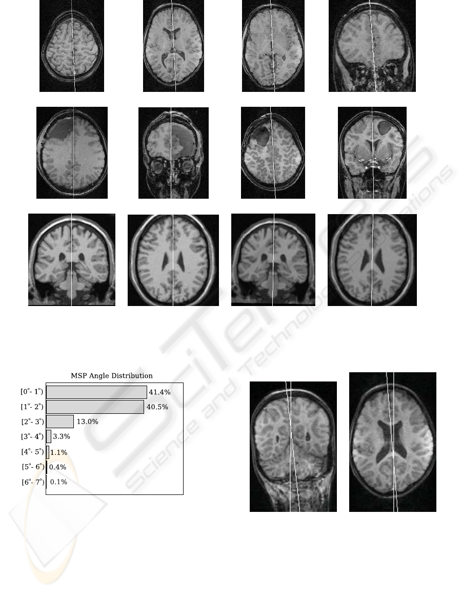
(a) (b) (c) (d)
(e) (f) (g) (h)
(i) (j) (k) (l)
Figure 5: Examples of planes computed by the method: (a–d): sample slices from a control dataset; (e–f) sample slices from
a surgery dataset; (g–h) sample slices from another surgery dataset; (i–j): sample slices from a phantom dataset; (k–l): sample
slices from a tilted dataset obtained from the one in (i–j).
Figure 6: Distribution of the angles between computed mid-
sagittal planes.
5 CONCLUSIONS AND FUTURE
WORK
We presented a fast and robust method for extrac-
tion of the mid-sagittal plane from MR images of the
brain. It is based on automatic segmentation of the
brain and on a heuristic search based on maximization
of CSF within the MSP. We evaluated the method on
(a) (b)
Figure 7: A coronal slice (a) and an axial slice (b) from
the case with maximum angular error (6.9
o
), with planes
in white: The fissure was thick at the top of the head, and
curved in the longitudinal direction, allowing the MSP to
snap either to the frontal or posterior segments of the fissure,
with some degree of freedom.
64 MR datasets, including images from patients with
large surgical cavities (Figure 2a and Figures 5e–h).
The method succeeded on all datasets and performed
FAST AND ROBUST MID-SAGITTAL PLANE LOCATION IN 3D MR IMAGES OF THE BRAIN
97
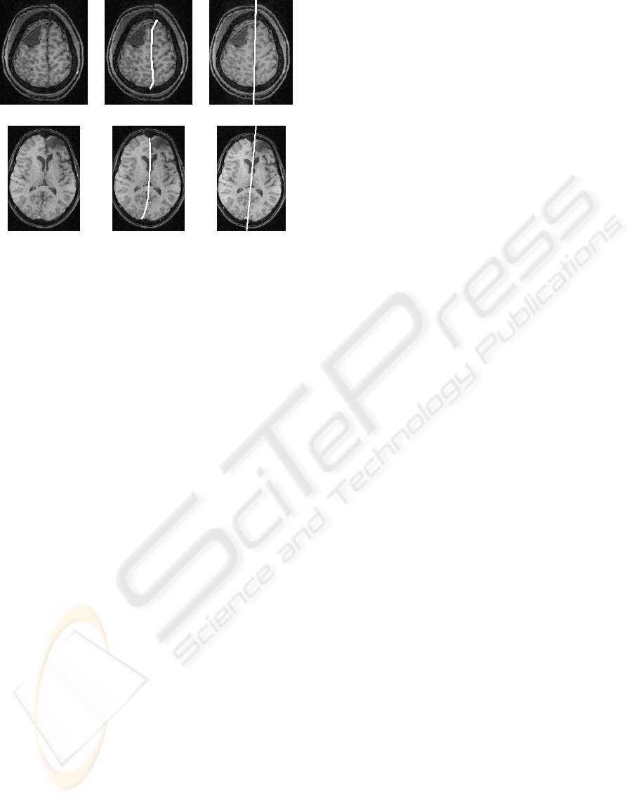
(a) (b) (c)
(d) (e) (f)
Figure 8: Non-planar fissures: (a) irregular fissure, (b) ex-
pert fissure delineation of (a) and (c) MSP computed by our
method. (d) Curved fissure, (e) expert fissure delineation of
(d) and (f) MSP computed by our method.
equally well on healthy and pathological cases. Ro-
tations and translations of the datasets led to mean
MSP variations around 1
o
, which is not a significant
error considering the discrete space of MR datasets.
MSP variations over 3
o
occurred only in cases where
the longitudinal fissure was not planar, and multiple
planes fitted different segments of the fissure with
similar scores. The method required a mean time of
60 seconds to extract the MSP from each MR dataset
on a common PC.
Previous fissure-based works were either evalu-
ated on images of healthy patients, on images with
small lesions (Volkau et al., 2006), or relied on local
symmetry measurements (Hu and Nowinski, 2003).
As future work, we intend to implement some of
the previous works and compare their accuracy and
performance with our method on the same datasets.
Brain mask computation is responsible for most of
the computing time. We also plan to evaluate how the
computation of the brain mask on lower resolutions
affect the accuracy and efficiency of the method.
ACKNOWLEDGEMENTS
The authors thank CAPES (Proc. 01P-05866/2007),
CNPq (Proc. 302427/04-0), and FAPESP (Proc.
03/13424-1) for the financial support.
REFERENCES
Ardekani, B., Kershaw, J., Braun, M., and Kanno, I. (1997).
Automatic detection of the mid-sagittal plane in 3-
D brain images. IEEE Trans. on Medical Imaging,
16(6):947–952.
Barrick, T. R., Mackay, C. E., Prima, S., Maes, F., Van-
dermeulen, D., Crow, T. J., and Roberts, N. (2005).
Automatic analysis of cerebral asymmetry: na ex-
ploratory study of the relationship between brain
torque and planum temporale asymmetry. NeuroIm-
age, 24(3):678–691.
Bergo, F. P. G., Falc˜ao, A. X., Miranda, P. A. V., and Rocha,
L. M. (2007). Automatic image segmentation by tree
pruning. Technical Report IC-07-23, Institute of Com-
puting, University of Campinas.
Brummer, M. E. (1991). Hough transform detection of
the longitudinal fissure in tomographic head images.
IEEE Trans. on Medical Imaging, 10(1):66–73.
Collins, D. L., Zijdenbos, A. P., Kollokian, V., Sled, J. G.,
Kabani, N. J., Holmes, C. J., and Evans, A. C.
(1998). Design and construction of a realistic digi-
tal brain phantom. IEEE Trans. on Medical Imaging,
17(3):463–468.
Crow, T. J. (1993). Schizophrenia as an anomaly of cere-
bral asymmetry. In Maurer, K., editor, Imaging of the
Brain in Psychiatry and Related Fields, pages 3–17.
Springer.
Csernansky, J. G., Joshi, S., Wang, L., Haller, J. W., Gado,
M., Miller, J. P., Grenander, U., and Miller, M. I.
(1998). Hippocampal morphometry in schizophrenia
by high dimensional brain mapping. Proceedings of
the National Academy os Sciences of the United States
of America, 95(19):11406–11411.
Csernansky, J. G., Wang, L., Joshi, S., Miller, J. P., Gado,
M., Kido, D., McKeel, D., Morris, J. C., and Miller,
M. I. (2000). Early DAT is distinguished from ag-
ing by high-dimensional mapping of the hippocam-
pus. Neurology, 55:1636–1643.
Davidson, R. J. and Hugdahl, K. (1996). Brain Asymmetry.
MIT Press/Bradford Books.
Falc˜ao, A. X., Bergo, F. P. G., and Miranda, P. A. V. (2004a).
Image segmentation by tree pruning. In Proc. of the
XVII Brazillian Symposium on Computer Graphics
and Image Processing, pages 65–71. IEEE.
Falc˜ao, A. X., Stolfi, J., and Lotufo, R. A. (2004b). The im-
age foresting transform: Theory, algorithms and appli-
cations. IEEE Trans. on Pattern Analysis and Machine
Intelligence, 26(1):19–29.
Geschwind, N. and Levitsky, W. (1968). Human brain:
Left-right asymmetries in temporale speech region.
Science, 161(3837):186–187.
Guillemaud, R., Marais, P., Zisserman, A., McDonald, B.,
Crow, T. J., and Brady, M. (1996). A three dimen-
sional mid sagittal plane for brain asymmetry mea-
surement. Schizophrenia Research, 18(2–3):183–184.
Highley, J. R., DeLisi, L. E., Roberts, N., Webb, J. A., Relja,
M., Razi, K., and Crow, T. J. (2003). Sex-dependent
BIOSIGNALS 2008 - International Conference on Bio-inspired Systems and Signal Processing
98

effects of schizophrenia: an MRI study of gyral fold-
ing, and cortical and white matter volume. Psychiatry
Research: Neuroimaging, 124(1):11–23.
Hogan, R. E., Mark, K. E., Choudhuri, I., Wang, L., Joshi,
S., Miller, M. I., and Bucholz, R. D. (2000). Mag-
netic resonance imaging deformation-based segmen-
tation of the hippocampus in patients with mesial tem-
poral sclerosis and temporal lobe epilepsy. J. Digital
Imaging, 13(2):217–218.
Hu, Q. and Nowinski, W. L. (2003). A rapid algorithm
for robust and automatic extraction of the midsagittal
plane of the human cerebrum from neuroimages based
on local symmetry and outlier removal. NeuroImage,
20(4):2153–2165.
Junck, L., Moen, J. G., Hutchins, G. D., Brown, M. B., and
Kuhl, D. E. (1990). Correlation methods for the cen-
tering, rotation, and alignment of functional brain im-
ages. The Journal of Nuclear Medicine, 31(7):1220–
1226.
Kapouleas, I., Alavi, A., Alves, W. M., Gur, R. E., and
Weiss, D. W. (1991). Registration of three dimen-
sional MR and PET images of the human brain with-
out markers. Radiology, 181(3):731–739.
Liu, Y., Collins, R. T., and Rothfus, W. E. (2001). Robust
midsagittal plane extraction from normal and patho-
logical 3D neuroradiology images. IEEE Trans. on
Medical Imaging, 20(3):175–192.
Liu, Y., Teverovskiy, L. A., Lopez, O. L., Aizenstein, H.,
Meltzer, C. C., and Becker, J. T. (2007). Discovery
of biomarkers for alzheimer’s disease prediction from
structural MR images. In 2007 IEEE Intl. Symp. on
Biomedical Imaging, pages 1344–1347. IEEE.
Mackay, C. E., Barrick, T. R., Roberts, N., DeLisi, L. E.,
Maes, F., Vandermeulen, D., and Crow, T. J. (2003).
Application of a new image analysis technique to
study brain asymmetry in schizophrenia. Psychiatry
Research, 124(1):25–35.
Minoshima, S., Berger, K. L., Lee, K. S., and Mintun,
M. A. (1992). An automated method for rotational
correction and centering of three-dimensional func-
tional brain images. The Journal of Nuclear Medicine,
33(8):1579–1585.
Miranda, P. A. V., Bergo, F. P. G., Rocha, L. M., and Falc˜ao,
A. X. (2006). Tree-pruning: A new algorithm and its
comparative analysis with the watershed transform for
automatic image segmentation. In Proc. of the XIX
Brazillian Symposium on Computer Graphics and Im-
age Processing, pages 37–44. IEEE.
Otsu, N. (1979). A threshold selection method from gray
level histograms. IEEE Trans. Systems, Man and Cy-
bernetics, 9:62–66.
Prima, S., Ourselin, S., and Ayache, N. (2002). Compu-
tation of the mid-sagittal plane in 3D brain images.
IEEE Trans. on Medical Imaging, 21(2):122–138.
Smith, S. M. and Jenkinson, M. (1999). Accurate robust
symmetry estimation. In Proc MICCAI ’99, pages
308–317, London, UK. Springer-Verlag.
Styner, M. and Gerig, G. (2000). Hybrid boundary-medial
shape description for biologically variable shapes. In
Proc. of IEEE Workshop on Mathematical Methods in
Biomedical Imaging Analysis (MMBIA), pages 235–
242. IEEE.
Sun, C. and Sherrah, J. (1997). 3D symmetry detection us-
ing the extended Gaussian image. IEEE Trans. on Pat-
tern Analysis and Machine Intelligence, 19(2):164–
168.
Talairach, J. and Tournoux, P. (1988). Co-Planar Sterio-
taxic Atlas of the Human Brain. Thieme Medical Pub-
lishers.
Teverovskiy, L. and Liu, Y. (2006). Truly 3D midsagittal
plane extraction for robust neuroimage registration. In
Proc. of 3rd IEEE Intl. Symp. on Biomedical Imaging,
pages 860–863. IEEE.
Tuzikov, A. V., Colliot, O., and Bloch, I. (2003). Evalua-
tion of the symmetry plane in 3D MR brain images.
Pattern Recognition Letters, 24(14):2219–2233.
Volkau, I., Prakash, K. N. B., Ananthasubramaniam, A.,
Aziz, A., and Nowinski, W. L. (2006). Extraction
of the midsagittal plane from morphological neuroim-
ages using the Kullback-Leibler’s measure. Medical
Image Analysis, 10(6):863–874.
Wang, L., Joshi, S. C., Miller, M. I., and Csernansky, J. G.
(2001). Statistical analysis of hippocampal asymme-
try in schizophrenia. NeuroImage, 14(3):531–545.
Wu, W.-C., Huang, C.-C., Chung, H.-W., Liou, M., Hsueh,
C.-J., Lee, C.-S., Wu, M.-L., , and Chen, C.-Y. (2005).
Hippocampal alterations in children with temporal
lobe epilepsy with or without a history of febrile
convulsions: Evaluations with MR volumetry and
proton MR spectroscopy. AJNR Am J Neuroradiol,
26(5):1270–1275.
FAST AND ROBUST MID-SAGITTAL PLANE LOCATION IN 3D MR IMAGES OF THE BRAIN
99
