RULE OPTIMIZING TECHNIQUE MOTIVATED BY HUMAN

CONCEPT FORMATION

Fedja Hadzic and Tharam S. Dillon

Digital Eciossytems and Business Intelligence Institute (DEBII), Curtin Universityof Technology, USA

Keywords: Data Mining, Rule Optimization, Feature Selection.

Abstract: In this paper we present a rule optimizing technique motivated by the psychological studies of human

concept learning. The technique allows for reasoning to happen at both higher levels of abstraction and

lower level of detail in order to optimize the rule set. Information stored at the higher level allows for

optimizing processes such as rule splitting, merging and deleting, while the information stored at the lower

level allows for determining the attribute relevance for a particular rule.

1 INTRODUCTION

During the rule optimization process a trade-off

usually needs to be made between the

misclassification rate (MR), and coverage rate (CR)

and generalization power (GP). MR corresponds to

the number of incorrectly classified instances and it

should be minimized. CR is the number of instances

that are captured by the rule set and this should be

maximized. Good GP is achieved by simplifying the

rules. The trade-off occurs especially when the data

set is characterized by continuous attributes where a

valid constraint on the attribute range needs to be

determined for a particular rule. Increasing the

attribute range usually leads to the increase in CR

but at the cost of an increase in MR. Similarly if the

rules are too general they may lack the specificity to

distinguish some domain characteristics and hence

the MR would increase.

In this paper we extend the rule optimizing

method presented in (Hadzic & Dillon, 2005; Hadzic

& Dillon, 2007). The method was used to optimize

the rules learned by a neural network and in this

work it is extended to be applicable to rules obtained

using any knowledge learning methods. The

extension allows reasoning to happen at both higher

level of abstraction and lower level of detail. The

information about the relationships between the

class attribute and the input attributes will be

available for determining the relevance of rule

attributes at any stage of the rule optimizing (RO)

process. The attributes irrelevant for a particular rule

can then be deleted. Furthermore, attributes

previously found as irrelevant can be re-introduced

if found relevant at a later stage in the process. The

proposed method is evaluated on the rules learned

from publicly available real world datasets and the

results indicate the effectiveness of the method.

2 MOTIVATION

Concept or category formation has been studied

extensively in the psychology area. Generally it

refers to the process by which a person learns to sort

specific observations into general rules or classes. It

allows one to respond to events in terms of their

class membership rather than uniqueness (Bruner et

al., 1956). This process is the elementary form by

which humans adjust to their environment. Relevant

attributes need to be identified and a rule has to be

learned, developed or applied for formulating a

concept (Sestito & Dillon, 1994). Human subjects

consistently seek confirming information by actively

searching they environment for appropriate

examples which can confirm or modify the newly

discovered concepts (Kristal 1981; Pollio 1974,

sestito & Dillon 1994). Hence, there exists one level

at which the concepts or categories have been

formed and there is another level where the

observations are used for confirming or adjusting the

learned concepts and their relationships (Rosch

1977). When a formed belief appears to be

contradictory for some observations one may go into

thinking at the lower level of detail to investigate the

constituents of that belief and what example

Hadzic F. and S. Dillon T. (2008).

RULE OPTIMIZING TECHNIQUE MOTIVATED BY HUMAN CONCEPT FORMATION.

In Proceedings of the First International Conference on Bio-inspired Systems and Signal Processing, pages 31-36

DOI: 10.5220/0001068300310036

 SciTePress

observations formed it. An update of the belief can

then occur whereby some pre-conditions are added

or removed from the constituents of that particular

belief. Re-introducing new features previously found

as irrelevant or removing the irrelevant one, can

occur quite frequently while learning occurs and

until some reliable belief is formed.

Being able to perform this type of task is

desirable for the rule optimizing process. The higher

level of abstraction would correspond to the rules

with the attribute constraints and the predicting class

values, while at the lower level the relationships

between attribute values and the occurring class

values are stored. This information can be used to

determine the relevance of attributes in predicting of

the class value that a particular rule implies.

Integrating the feature selection criterion with the

rule optimizing stage is advantageous since initial

bad choices made about the attribute relevance could

be corrected as learning proceeds.

3 METHOD DESCRIPTION

The method takes as input a file describing the rules

detected by a particular classifier and the domain

dataset from which the rules were learned. The rules

are represented in a graph structure (GS) where each

rule has a set of attribute constraints and points to

one or more target values. The GS contains the high

level information about the domain at hand in form

of rules and is used for reasoning at the higher level

of abstraction.

3.1 Graph Structure Formation

In order for the GS to be formed two files are read,

one describing the rules detected by a classifier and

the other containing the total set of instances from

which the rules were learned. The rules are in form

of attribute constraints while the implying class of

each rule is ignored. The reason is that during the

whole process of RO, the implying class values can

change as some clusters will be merged or split.

Rather the domain dataset is read according to which

the weighted links between the rules and class

values are set. The implying class value of a rule

becomes the highest weighted link to a particular

class value node. This class value has most

frequently occurred in the instances which were

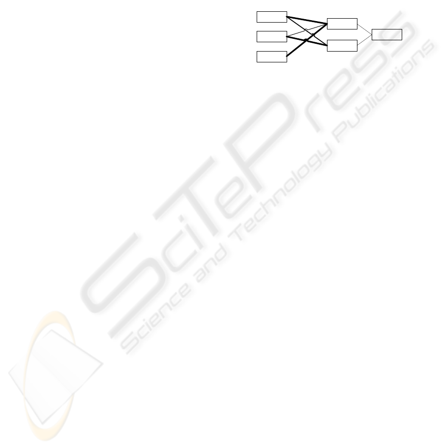
captured by the rule. An example of the GS after a

dataset is read in is shown in Figure 1. The implying

class of Rule1 and Rule 3 would be class value 1

while for Rule2 it is class value 2. Even though it is

not shown in the figure, each rule has a set of

attribute constraints associated with it, which we

refer to as the weight vector (WV) of that rule. The

set of attribute values occurring in the instance being

processed are referred to as the input vector (IV).

Hence, to classify an instance we match the IV

against the WVs of the available rules. A constraint

for a continuous attribute is given in terms of a

lower range (lr) and an upper range (ur) indicating

the set of allowed attribute values.

Rule1

Rule2

Rule3

Class

Value2

Value1

Figure 1: Example graph structure from high level.

3.2 Storing Lower Level Information

Previous sub-section has explained the GS formation

at the top level which is used mainly for determining

the implying class values of the rules. In this section

we discuss how lower level instance information is

stored for each rule. This low level information is

necessary for the reasoning at the lower level.

As previously mentioned each rule has a set of

attribute constraints associated with it, which are

stored in its WV. For each of the attributes in the WV

we collect the occurring attribute values in the

instances that were captured by that particular rule.

Hence each attribute has a value list (VL) associated

with it which stores all the occurring attribute

values. Furthermore, each of the value objects in the

list has a set of weighted links to the occurring class

values in the instance where that particular value

occurred. This is necessary for the feature selection

process which will be explained later. For a

continuous attributes there could be many occurring

values and values close to one another are merged

into one value object when the difference between

the values is less than a chosen merge value

threshold. Hence the numerical values stored in a list

of a continuous attribute will be ordered so that a

new value is always stored in an appropriate place

and the merging can occur if necessary. Figure 2

illustrates how this low level information is stored

for a rule that consists of two continuous attributes A

and B. The attribute A has the lower range (lr) and

the upper range (ur) in between which the values v1,

v2 and v3 occur. The ‘lr’ of A is equal to the value

of v1 or the ‘lr; of v1 if v1 is a merged value object,

BIOSIGNALS 2008 - International Conference on Bio-inspired Systems and Signal Processing

while the ‘ur’ of A is equal to the value of v3 or the

‘ur’ of v3 if v3 is a merged value object.

A B

lr u r

v1 v2 v3 v1 v2

Class

Value2Value1

lr u r

Figure 2: Storing low level instance information.

3.3 Reasoning at the Higher Level

Once the implying classes are set for each of the

rules the dataset is read in again in order to check for

any misclassifications and update the rule set

accordingly. When a rule captures an instance that

has a different class value than the implication of the

rule, a child rule will be created in order to isolate

the characteristic of the rule causing the

misclassification. The attribute constraints of the

parent and child rule are updated so that they are

exclusive from one another. The child attribute

constraint ranges from the attribute value of the

instance to the range limit of the parent rule to which

the input attribute value was closest to. The parent

rule adopts the remaining range as the constraint for

the attribute at hand.

After the whole dataset is read in there could be

many child rules created from a parent rule. Some

child rules may be merged together first but

explanation of this is to come later once we discuss

the process of rule similarity comparison and

merging. If a child rule points to other target values

with high confidence it become a new rule and this

corresponds to the process of rule splitting, since the

parent rule has been modified to exclude the child

rule which is now a rule on its own. On the other

hand if the child rule still mainly points to the

implying class value of the parent rule it is merged

back into the parent rule (if they are still similar

enough). An example of a rule which has been

modified to contain a few children due to the

misclassifications is displayed in Figure 3. The

reasoning explained would merge ‘Child3’ back into

the parent rule since it points to the implying class of

the parent rule with high weight. This is assuming

that they are still similar enough. On the other hand

Child1 and Child2 would become new rules since

they more frequently capture the instances where the

class value is different to the implying class of the

parent rule. Furthermore if they are similar enough

they would be merged into one rule.

Rule

Child1

Child2

Child3

Class

Value2

Value1

Figure 3: Example of rule splitting.

In order to measure the similarity among the

rules we make use of a modified Euclidean distance

(ED) measure. This measure is also used to

determine which rule captures a presented instance.

An instance is always assigned to the rule with the

smallest ED to the IV. Even though one would

expect the ED to be equal to 0 when classifying

instances this may not always be the case throughout

the RO process. The ED calculation is calculated

according to the difference in the allowed range

values of a particular attribute. The way that ED is

calculated is what determines the similarity among

rules, and therefore we first overview the ED

calculation and then proceed onto explaining the

merging of rules that may occur in the whole RO

process.

3.3.1 ED Calculation

For a continuous attribute a

occurring at the position

i of WV of rule R, let ‘a

lr’ denote the lower range,

‘a

ur’ the upper range, and ‘a

v’ the initial value if

the ranges of a

are not set. The value from the i-th

attribute of IV will be denotes as iva

. The i-th term

of the ED calculation between IV and WV of R for

continuous attributes is:

- case 1: a

ranges are not set

• 0 iff iva

= a

• iva

- a

v if iva

> a

• a

v - iva

if iva

< a

- case 2: a

ranges are set

• 0 iff iva

≥ a

lr and iva

≤ a

• a

lr - iva

if iva

< a

• iva

- a

ur if iva

> a

The input merge threshold used for continuous

attribute (MT) also needs to be set with respect to the

number of continuous attributes in the set. It

corresponds to the maximum allowed sum of the

range differences among the WV and IV so that the

rule would capture the instance at hand.

RULE OPTIMIZING TECHNIQUE MOTIVATED BY HUMAN CONCEPT FORMATION

When calculating the ED for the purpose of

merging similar rules there are four possibilities that

need to be accounted with respect to the ranges

being set in the rule attributes, and the ED

calculation is adjusted. For rule R

let r

denote the

attribute occurring at the position i of WV of rule R

let ‘r

lr’ denote the lower range, ‘r

ur’ the upper

range, and ‘r

v’ the initial value if the ranges of r

are not set. Similarly for rule R

let r

denote the

attribute occurring at the position i of WV of rule R

let ‘r

lr’ denote the lower range, ‘r

ur’ the upper

range, and ‘r

v’ the initial value if the ranges of r

are not set. The i-th term of the ED calculation

between the WV of R

and WV of R

for continuous

attributes is:

- case 1: both r

and r

ranges are not set

• 0 iff r

v = r

• r

v - r

v if r

v > r

• r

v - r

if r

v < r

- case 2: r

ranges are set and r

ranges are not set

• 0 iff r

v ≥ r

lr and r

v ≤ r

• r

lr - r

v if r

v < r

• r

v – r

ur if r

v > r

- case 3: r

ranges are not set and r

ranges are set

• 0 iff r

v ≥ r

lr and r

v ≤ r

• r

lr – r

v if r

v < r

• r

v – r

ur if r

v > r

- case 4: both r

and r

ranges are set

• 0 iff r

lr ≥ r

lr and r

ur ≤ r

• 0 iff r

lr ≥ r

lr and r

ur ≤ r

• min(r

lr - r

lr, r

ur - r

ur) iff r

lr >

lr and r

ur > r

• min(r

lr - r

lr, r

ur -r

ur iff r

lr >

lr and r

ur > r

• (r

lr – r

ur) iff r

lr > r

• (r

lr – r

ur) iff r

lr > r

For a rule to capture an instance or for it to be

considered sufficiently similar to another rule the

ED would need to be smaller than the MT threshold.

3.3.2 Rule Merging

As mentioned at the start of Section 3.3 the child

rules may be created when a particular rule captures

an instance that has a different class value than the

implying class value of that rule (i.e.

misclassification occurs). After the whole file is read

in the child rules that have the same implying class

values are merged together if the ED between them

is below the MT. Thereafter the child rules either

become a new rule or are merged back into the

parent rule, as discussed earlier. Once all the child

rules have been validated the merging can occur

among the new rule set. Hence if any of the rules

have the same implying class value and the ED

between them is below the MT the rules will be

merged together and the attribute constraints

updated. After this process the file is read in again

and any of the rules that do not capture any instances

are deleted form the rule set.

3.4 Reasoning at the Lower Level

Once the rules have undergone the process of

splitting and merging, the relevance of rule attributes

should be calculated as some attributes may have

lost their relevance through merging of two or more

rules. Other attributes may have become relevant as

a more specific distinguishing factor of a new rule

which resulted from splitting of an original rule. For

this purpose we make use of the symmetrical tau

(Zhou & Dillon, 1991) feature selection criterion

whose calculation is made possible by the

information stored at the lower level of the graph

structure. We start this section by discussing the

properties of the symmetrical tau and then proceed

onto explaining how the relevance cut-off is

determined and the issue of choosing the merge

value threshold for the value objects in a value list.

3.4.1 Feature Selection Criterion

Symmetrical Tau (τ) (Zhou & Dillon, 1991) is a

statistical measure for the capability of an attribute

in predicting the class of another attribute. The τ

measure is calculated using a contingency table

which is used in statistical area to record and analyze

the relationship between two or more variables. If

there are I rows and J columns in the table, the

probability that an individual belongs to row

category i and column category j is represented as

P(ij), and P(i+) and P(+j) are the marginal

probabilities in row category i and column category j

respectively, the Symmetrical Tau measure is

defined as (Zhou & Dillon, 1991):

For the purpose of feature selection problem one

criteria in the contingency table could be viewed as

an attribute and the other as the target class that

needs to be predicted. In our case the information

contained in a contingency table between the rule

attributes and the class attributes is stored at the

BIOSIGNALS 2008 - International Conference on Bio-inspired Systems and Signal Processing

lower level of the graph structure as explained in

Section 3.2. The τ measure was used as a filter

approach for the feature subset selection problem in

(Hadzic & Dillon, 2006). In the current work its

capability of measuring the sequential variation of

an attribute’s predictive capability is exploited.

3.4.2 Determining Relevance Cut-off

For each of the rules that are triggered for multiple

class values we calculate the τ criterion and rank the

rule attributes according to the decreasing τ value.

The relevance cut-off point is determined as the

point in the ranking where the τ value of an attribute

is less than half of the previous attribute’s τ value.

All the attributes below the cut-off point are

considered irrelevant for that particular rule and are

removed from the rule’s WV. On the other hand, if

some of the attributes above the relevance cut-off

point were previously excluded from the WV of the

rule, they are now re-introduced since their τ value

indicates their relevance for the rule at hand.

As mentioned in Section 3.2 when the occurring

values stored in the value list of an attribute are

close together they are merged and the new value

object represents a range of values. The merge value

threshold chosen determines when the difference

among the value objects is sufficiently small for

merging to occur. This is important for appropriate τ

calculation. Ideally a good merge value threshold

will be picked with respect to the value distribution

of that particular attribute. However, this

information is not always available and in our

approach we pick a general merge threshold of

around 0.02. This has some implications for the

calculated τ value since when the categories of an

attribute A are increased more is known about

attribute A and the error in predicting attribute B

may decrease. Hence, if the merge value threshold is

too large many attributes will be considered as

irrelevant since all the occurring values could be

merged into one value object which points to many

target objects and this aspect would indicate no

distinguishing property of the attribute. On the other

hand, if it is too small many value objects may exist

which may wrongly indicate that the attribute has

high relevance in predicting the class attribute.

4 METHOD EVALUATION

The proposed method was evaluated on two rule sets

learned from publicly available real world datasets

(Blake et al., 1998). The rule optimizing process was

run for 10 iterations for each of the tested domains.

The first set of rules we consider has been

learned from the ‘Iris’ dataset using the continuous

self-organizing map (Hadzic & Dillon, 2005) so that

we can compare the improvement of the extension to

the rule optimizing method. The merge cluster

threshold MT was set to 0.1 and the merge value

threshold MVT for attribute values was set to 0.02.

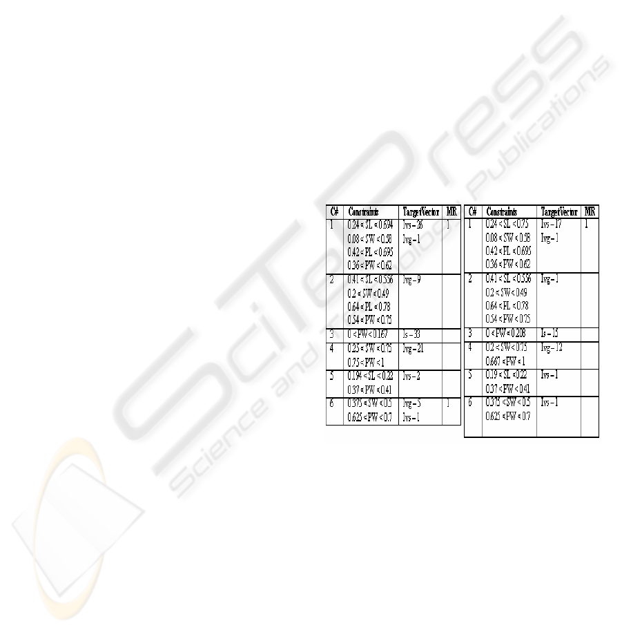
The rules obtained using the CSOM technique

(Hadzic & Dillon, 2005) are displayed in Figure 4.

When the rules obtained after retraining were taken

as input by our proposed rule optimization method

the resulting rule set was different in only one rule.

The rule 4 was further simplified to exclude the

attribute constraint from sepal-width and the new

attribute constraint was only that petal-width has to

be between the values of 0.667 and 1.0 for the class

value of Iris-virginica. Hence the process was able to

detect another attribute that has become irrelevant

during the RO process. The predictive accuracy

remained the same.

Figure 4: Iris rule set as obtained by using the traditional

rule optimizing technique.

With respect to using CSOM to extract rules

from the ‘Iris’ domain we have performed another

experiment. The initial rules extracted by CSOM

without the network pruning and retraining of the

network were optimized. When network pruning

occurs the network should be re-trained for new

abstractions to be properly formed. In this

experiment we wanted to see how the RO technique

performs by itself without any network pruning or

retraining.

RULE OPTIMIZING TECHNIQUE MOTIVATED BY HUMAN CONCEPT FORMATION

Rules Implying class

0.33 < PL < 0.678

0.375 < PW < 0.792

Iris-versicolor

0.208 < SW < 0.542

0.627 < PL < 0.847

0.54 < PW < 1.0

Iris-virginica

0.778 < SL < 1.0

0.25 < SW < 0.75

0.814 < PL < 1.0

0.625 < PW < 0.917

Iris-virginica

0.0 < SL < 0.417

0.41 < SW < 0.917

0.0 < PL < 0.153

0.0 < PW < 0.208

Iris-setosa

Figure 5: Optimized initial rules extracted by CSOM

Notation: SL – sepal_length, SW – sepal_width, PL –

petal _length, PW – petal_width.

By applying the RO technique the rule set was

reduced to four rules as displayed in Figure 5.

However, not as many attributes were removed from

each of the rules and two instances were

misclassified. Hence, performing network pruning

and retraining prior to RO may achieve a more

optimal rule set. However, in the cases where

retraining the network may be too expensive the RO

technique can be applied by itself. In fact compared

to the initial set of rules detected by CSOM, which

consisted of nine rules with three misclassified

instances this is still a significant improvement.

The second set of experiments was performed on

the complex ‘Sonar’ dataset which consists of sixty

continuous attributes. The examples are classified

into two groups one identified as rocks (R) and the

second identified as metal cylinders (M). The

learned decision tree by the C4 algorithm (Quinlan,

1990) consisted of 18 rules with the predictive

accuracy equal to 65.1%. These rules were taken as

input in our RO technique and the MT was set to 0.2

while the MVT was set to 0.0005. The optimized rule

set consisted of only two rules i.e 0.0 < a11 <= 0.197

Æ R and 0.197 < a11 <= 1.0 Æ M. When tested on

an unseen dataset the predictive accuracy was 82.2

% i.e. 11 instances were misclassified from the

available 62. Hence the RO process has again proved

useful in simplifying the rules set without the cost of

increasing the number of misclassified instances.

5 CONCLUSIONS

This paper has presented a rule optimizing technique

motivated by the psychological studies of human

concept information. The capability to swap from

the higher level reasoning to the reasoning at the

lower instance level has indeed proven useful for

determining the relevance of attributes throughout

the rule optimizing process. The method is

applicable to the optimization of rules obtained from

any data mining techniques. The evaluation of the

method on the rules learned from real world data by

different classifier methods has shown its

effectiveness in optimizing the rule set. As a future

work method needs to be extended so that

categorical attributes can be handled as well.

Furthermore, it would be interesting to explore the

possibilities of the rule optimizing method in

becoming a stand-alone machine learning method

itself.

REFERENCES

Blake, C., Keogh, E. and Merz, C.J., 1998. UCI

Repository of Machine Learning Databases, Irvine,

CA: University of California, Department of

Information and Computer Science., 1998.

[http://www.ics.uci.edu/~mlearn/MLRepository.html].

Bruner, J.S., Goodnow, J.J., and Austin, G.A., 2001. A

study of thinking, John Wiley & Sons, Inc., New York,

1956.

Hadzic, F. & Dillon, T.S., 2005. “CSOM: Self Organizing

Map for Continuous Data”, 3

Int’l IEEE Conf. on

Industrial Informatics, 10-12 August, Perth.

Hadzic, F. and Dillon, T.S., 2006 “Using the Symmetrical

Tau (τ ) Criterion for Feature Selection in Decision

Tree and Neural Network Learning”, 2

Workshop on

Feature Selection for Data Mining: Interfacing

Machine Learning and Statistics, in conj. with SIAM

Int’l Conf. on Data Mining, Bethesda, 2006.

Hadzic, F. & Dillon, T.S., 2007. “CSOM for Mixed Data

Types”, 4

Int’l Symposium on Neural Networks, June

3-7, Nanjing, China.

Kristal, L., ed. 1981, ABC of Psychology, Michael Joseph,

London, pp. 56-57.

Pollio, H.R., 1974, The psychology of Symbolic Activity,

Addison-Wesley, Reading, Massachusetts.

Quinlan, J.R., 1990. “Probabilistic Decision Trees”,

Machine Learning: An Artificial Intelligence

Approach Volume 4, Kadratoff, Y & Michalski, R.,

Morgan Kaufmann Publishers, Inc., San Mateo,

California.

Roch, E. 1977, “Classification of real-world objects:

Origins and representations in cognition”, in Thinking:

Readings in Cognitive Science, eds P.N. Johnson-

Laird & P.C. Wason, Cambridge University Press,

Cambridge, pp. 212-222.

Sestito, S. and Dillon, S.T., 1994. Automated Knowledge

Acquisition. Prentice Hall of Australia Pty Ltd,

Sydney.

Zhou, X., and Dillon, T.S., 1991. “A statistical-heuristic

feature selection criterion for decision tree induction”,

IEEE Transactions on Pattern Analysis and Machine

Intelligence, vol. 13, no.8, August, pp 834-841.

BIOSIGNALS 2008 - International Conference on Bio-inspired Systems and Signal Processing