
DIMENSIONALITY REDUCTION FOR IMPROVED SOURCE
SEPARATION IN FMRI DATA
Rudolph L. Mappus IV, David Minnen and Charles Lee Isbell Jr.
College of Computing, Georgia Tech, 85 Fifth St. NW, Atlanta, USA
Keywords:
Dimensionality reduction, ICA, fMRI.
Abstract:
Functional magnetic resonance imaging (fMRI) captures brain activity by measuring the hemodynamic re-
sponse. It is often used to associate specific brain activity with specific behavior or tasks. The analysis of
fMRI scans seeks to recover this association by differentiating between task and non-task related activation
and by spatially isolating brain activity. In this paper, we frame the association problem as a convolution of
activation patterns. We project fMRI scans into a low dimensional space using manifold learning techniques.
In this subspace, we transform the time course of each projected fMRI volume into the frequency domain. We
use independent component analysis to discover task related activations. The combination of these methods
discovers sources that show stronger correlation with the activation reference function than previous methods.
1 INTRODUCTION
Functional magnetic resonance imaging (fMRI) cap-
tures neural activation patterns by measuring the
hemodynamic response in cranial tissue through sam-
pling discrete regions of the brain, referred to as vox-
els (Dogil et al., 2002). Each voxel represents the
aggregate hemodynamic response of a region of neu-
rons. Behavioral experiments using fMRI are de-
signed to evoke activation in a hypothesized region
of interest (ROI) in the brain. The ROI represents an
anatomical region of the brain believed to be where
functional processing of a specific behavioral task oc-
curs. Experimental trials in these designs use a be-
havioral task meant to evoke activation in the ROI.
Control trials do not evoke ROI activation.
Unfortunately, locating significant differences be-
tween active and non-active voxels is challenging be-
cause of the inherent latencies and artifacts in fMRI
signal acquisition (Josephs et al., 1997). Furthermore,
the hemodynamic activation level of neighboringvox-
els influences voxel activation, producing less accu-
rate spatial activation maps.
Traditional analysis methods such as statistical
parametric mapping (SPM) use statistical tests to
demonstrate significant differences between the time
course activation of particular voxels in the control
and experimental tasks (Friston, 2003). By con-
trast, the objective of component analysis methods—
such as independent components analysis (ICA)—
is to recover components whose time course activa-
tion correlates with the task-based reference function:
argmax
a∈{A}
ρ(r, a), where r is the reference activa-
tion time course that represents the ideal activation
during the trial, and a is the component activation
time course.
Although ICA has been shown to work for simple
block experimental designs, it has some limitations.
In particular, ICA has been used successfully when
combined with a priori anatomical information about
activation areas (McKeown et al., 1998). Further-
more, simple ICA does not account for the delayed
composition effects that can arise in fMRI analysis.
The contribution of this work is to frame the prob-
lem of the combined latencies of the hemodynamic
response and the signal acquisition process as a con-
volution of the hemodynamic response functions of
spatially independent components. Framed this way,
we can address these confounding spatial and tem-
poral influences, by first using nonlinear manifold
learning to constrain source separation and to remove
voxels that do not help distinguish between task and
non-task activation. We generate a frequency space
representation of the reduced features for convolutive
source separation using ICA. Our method allows us to
handle delayed composition effects and to select ROIs
308
L. Mappus IV R., Minnen D. and Lee Isbell Jr. C. (2008).
DIMENSIONALITY REDUCTION FOR IMPROVED SOURCE SEPARATION IN FMRI DATA.
In Proceedings of the First International Conference on Bio-inspired Systems and Signal Processing, pages 308-313
DOI: 10.5220/0001068403080313
Copyright
c
SciTePress

without specific a priori anatomical knowledge of the
ROI. Thus, we are able to limit type II errors.
2 PREVIOUS WORK
Independent Components Analysis. Time domain
independent component analysis (ICA) works on dis-
crete time, linear dynamical systems where a latent
process generates a set of observables (McKeown
et al., 1998). A k-vector of random variables rep-
resents the state of the process at each time step.
In such a system, latent variables are linearly mixed
to give rise to the observable variables at each time
step. First-order Markov dynamics govern state tran-
sitions within the process defined by a k × k matrix
M (Roweis and Ghahramani, 1999).
Formally, X = AS, where X is a k × t observa-
tion matrix, A is a mixing matrix and S is the k × t
matrix representing the time course evolution of the
latent random variables. ICA recovers an unmixing
matrix A
−1
for the observation matrix X. A
−1
pro-
duces a set of statistically independent components
from the data. Under certain assumptions, the com-
ponents represent the (possibly scaled) evolution of
the original latent process. In this case, the mixing
matrix A represents the degree to which a component
participates in the generation of the observation data
at each time step. For the analysis of fMRI scans, we
assume that the separation problem in the reduced di-
mension problem is determined, which means that the
number of sources is equal to the number of sensors
(voxels). In the determined case, the discovered inde-
pendent components can be interpreted as underlying
causes of observations, especially when one believes
that: (1) observed features are generated by the in-
teraction of a set of independent hidden random vari-
ables, and (2) these hidden variables are likely to be
kurtotic (i.e. discriminative and sparse). These as-
sumptions are reasonable for fMRI analysis because
of existing neurological evidence for functional mod-
ularity in the brain and the specific requirements of
the experimental task.
Time domain applications of ICA assume an in-
stantaneous linear mixture model at each time step.
McKeown et al. (McKeown et al., 1998) applied ICA
to fMRI data from a simple block-design experiment
and found correlated activation signal for a compo-
nent corresponding to the region of interest (McKe-
own et al., 1998).
Manifold Learning and fMRI. Manifold learning
has been applied to fMRI time domain data directly
(Shen and Meyer, 2006). In this case, the intrinsic
dimensionality represents spatially independent voxel
activations and the objective is to generate clusters
matching ground truth classification. The intuition is
that task related activated voxels will cluster together
in the representation. The interpretation of the mani-
fold is that it captures information about the geometry
of the volume space. A key issue with direct appli-
cation is that target signals in a behavioral study are
often not the high ranking elements generated using
principle components analysis (PCA) and ICA (McK-
eown et al., 1998). These less significant activations
typically rank in the latter component quartiles.
Convolutional Blind Source Separation. Blind sep-
aration of convolutional sources has applications in
a number of signal processing domains, including
fMRI (Pederson et al., 2007; Anemuller et al., 2003).
Here, we assume a linear convolution of sources in
the time domain and model observations at time t as:
x(t) =
K−1
∑
k=0
A
k
s(t − k) + v(t) (1)
where K is the finite impulse response (FIR) length.
In frequency space, source separation is performed
for each frequency. For the purpose of analyzing
fMRI data, where there is a relatively limited tempo-
ral extent, we choose a window function that mini-
mizes band overlap.
W(ω) = A(ω)S(ω) + V(ω) (2)
3 COMBINED APPROACH
Our approach to fMRI analysis seeks to combine the
strengths of manifold learning, convolution in fre-
quency space, and complex ICA in order to improve
the accuracy of recovered brain activity components.
Manifold learning has not been applied to time do-
main data as preprocessing for component analysis.
Furthermore, manifold learning techniques reduce the
dimensionality of the ROI, making component analy-
sis more effective at source separation. In fact, much
of the ROI is not significantly activated and correlated
to the reference function. We want to reduce the di-
mensionality of these voxels before source separation.
Using ICA in the frequency domain allows us to
treat convolution of components as a product, which
in turn allows a computationally feasible algorithm
to solve the convolutive blind source separation prob-
lem. Using this version of the source separation prob-
lem is important because voxels near each other in the
brain may exhibit delayed influences during record-
ing. Using a convolutive model instead of an instan-
taneous mixing model provides the ability to capture
this influence and properly separate the components.
DIMENSIONALITY REDUCTION FOR IMPROVED SOURCE SEPARATION IN FMRI DATA
309

3.1 Manifold Learning
Before transformation into the frequency domain and
subsequent component analysis, we apply a manifold
learning algorithm to reduce the size of the voxel
set. The dimensionality reduction serves two pur-
poses. First, it reduces the computational burden of
the relatively expensive ICA computation. More im-
portantly, manifold learning allows researchers to in-
clude a large ROI in order to avoid Type II errors
caused by failing to include a relevant voxel in the
analysis. The dimensionality reduction algorithm can
then reduce the region based on the observed activa-
tion levels, thereby achievinga manageable size while
minimizing the risk of excluding relevant voxels.
We experiment with several different mani-
fold learning methods: local linear embedding
(LLE) (Roweis and Saul, 2000), isomap (Tenen-
baum et al., 2000), Laplacian eigenmaps (Belkin and
Niyogi, 2003) and diffusion maps (Coifman and La-
fon, 2006). Diffusion maps were used in previous
work with fMRI (Shen and Meyer, 2006), while LLE
and isomap are both standard methods for manifold
learning and provide a basis for comparison.
3.2 Complex ICA
In order to convert the time course of voxel activa-
tions into the frequency domain, we use the short–
time Fourier transform (STFT) with a window size
adapted for each dataset. In the case of the left/right
dataset (described in detail in the following section),
the window size equals the ratio of the hemody-
namic response latency to volume acquisition latency.
Each STFT generates frequency vectors for a spe-
cific temporal window, which are grouped into fre-
quency vectors and analyzed via complex ICA. The
Fourier transforms represent signals in each bin in
the frequency domain as complex values. We apply
complex-fastICA (Bingham and Hyvarinen, 2000) to
each bin, so that the generated components are fre-
quency specific.
3.3 Component Comparison
We select components with activation sharing high
correlation to the reference activation function. We
consider these components to be task related. In the
time domain, application of ICA generates the acti-
vation of independent sources in the columns of the
unmixing matrix A, and correlation of these columns
to the reference function indicates task relatedness. In
the frequency domain, where there STFT generates a
set of frequency bins, the objective is to find com-
ponents in each frequency bin that are task related.
We generate the reference activation function using
the same parameters (same spectral extent, same bin
parameters) used to generate the STFT for the obser-
vation set. We use the standard distance measure for
complex vectors:
∑
i
|x|
2
. For each bin, we find the
highest correlated activation course: argmax
a
ρ(a, r).
4 EXPERIMENTS
Here, we present results of experiments comparing
performance of the manifold learning techniques and
complex source separation alone. The datasets are
meant to demonstrate method performance in a sim-
ple, controlled task as well as actual study data.
4.1 Left/right Motor Task
To evaluate our method, we begin with a simple ex-
ample: consider an fMRI scan sequence of a single
subject performing a repetitive right- or left-hand fin-
ger movement task (Hurd, 2000). The objective is to
find task related activated components of hand move-
ments in the ROI. For the ROI, we selected a window
of voxels in a region based on correlation values to the
reference function using time domain ICA. In the mo-
tor task, 80 volumes were sampled at a constant rate
for each task: left-hand/right-hand finger move. We
defined a ROI in slices 13,14,15,16, loosely defined
around the temporal area of the motor cortex. Scans
of left hand tasks are concatenated to scans of right
hand tasks, 160 scans total. Given this organization,
the reference activation function for left hand tasks is
defined as a delta function: δ(x ≥ 80).
First, we want to test how manifold learning tech-
niques assist in time domain separation. In this case,
we compare the correlation of component activations
recovered by ICA to reference function activation.
We compare the best correlation values generated us-
ing ICA alone as well as with the various manifold
learning techniques. These are all performed using
the time domain data (see Table 1). The manifold
learning methods do not recover correlated activation
of components as well as using ICA alone in this case.
For the STFT, we use a parameterization for each
dataset. In the case of the left/right dataset, the win-
dow size is the ratio of the hemodynamic response la-
tency to volume acquisition latency. We consider the
measured values of voxels v
i
through time t
i∈{1...τ}
.
Each STFT generates frequency vectors for each win-
dow. We group frequency vectors from each STFT
and apply component analysis to the resulting matri-
ces. Computing the inverse transform of the compo-
BIOSIGNALS 2008 - International Conference on Bio-inspired Systems and Signal Processing
310
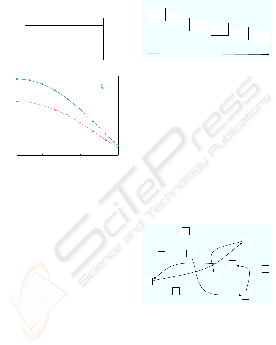
Table 1: Comparison of correlation values to reference
function using manifold learning in time domain.
Method Max ρ p-value
Diff Map 0.1407 0.1
Isomap 0.3470 0.001
LLE 0.2052 0.01
LE 0.2236 0.005
ICA 0.7395 0.0001
1 2 3 4 5 6 7 8 9
0
2
4
6
8
10
12
14
Frequency Bin
Min Dist to Reference Function
cICA
Diff Map
Isomap
LLE
Figure 1: Comparison of minimum distances to reference
function between manifold learning method preprocessing
and complex ICA. Minimum distance for each method in
each STFT frequency bin.
nent produces a time domain representationof the sig-
nal. However, due to the window overlap in the STFT,
this time scale is not appropriatefor comparisonin the
original observation space.
We compare the performance in the left/right task
between the various manifold learning algorithms and
complex ICA in the frequency domain without mani-
fold learning (see Table 1). To compare methods, we
use the minimum distance of component activation to
reference function activation in each frequencybin. In
this case, manifold learning using diffusion maps and
local linear embedding perform slightly better than
complex ICA alone.
4.2 Postle et Al. Study
Postle et al. (Postle et al., 2000) measured activation
of five participants in four behavioral tasks: forward
memory, manipulate memory, guided saccade, and a
free saccade task. Subjects completed 96 trials: 8
blocks of 12 trials each. Within each block, subjects
received an equal number of task trials, in random or-
der. Subjects were presented with a static arrange-
ment of squares on a screen. Signals were acquired
using a GE 1.5T scanner with 3.75mm
2
in-plane res-
Initial Instructions
500 msec
ISI
500 msec
Encoding/Guided
Saccades
6 sec
Pre-delay
Instructions
1 sec
Delay
7 sec
Probe
2 sec
Time
Figure 2: Trial event sequence (Postle et al., 2000). Initial
instructions indicate what the memory task will be. After
ISI, a sequence of highlighted boxes (see Figure 3) or fixa-
tion points appear. Pre-delay instructions indicate whether
the memory task is “forward,” “down to up,” or “fixate.”
After the delay, the probe is shown.
olution and 5mm inter-slice distance. Volumes were
21 slices, and volume acquisition time was 2s; 17 vol-
umes were acquired per trial. Inter-trial time was 7s.
By comparing voxel activation values in each experi-
mental task in the ROI, Postle et al. showed no signif-
icant difference in voxel activations between control
and experimental tasks.
Figure 2 shows the trial sequence. First, subjects
are told what the trial task will be: “memory,” “no
memory,” or “free eye movements.” Following an in-
terstimulus interval (ISI) of 500ms, subjects receive
the sequence of highlighted squares (Figure 3) fol-
lowed by further instructions: “forward,” “down-to-
up,” or “fixate.” After the return to baseline delay,
subjects receive the probe: a highlighted square in the
sequence.
5
1
4
6
3
2
Figure 3: Memory task stimulus. A fixed number of squares
are oriented on a screen. During memory tasks, a sequence
of the squares are highlighted in a random order. An exam-
ple highlight sequence for memory is shown.
Behavioral Tasks. During forward memory, manip-
ulate memory, and guided saccade tasks, a sequence
of squares was highlighted followed by a delay and
then a task prompt (see Figures 2&3). In forward
memory tasks, subjects were presented a sequence of
highlighted squares. Then, given one of highlighted
DIMENSIONALITY REDUCTION FOR IMPROVED SOURCE SEPARATION IN FMRI DATA
311

Table 3: Comparison of minimum distances to reference function activation between manifold learning methods in combina-
tion with complex ICA and complex ICA alone. For each bin (columns), the minimum distance for each method is shown
(i.e. the distance of the best matching components in each frequency bin).
1 2 3 4 5 6 7 8 9
Subject H
ICA 30.9077 29.5631 28.0292 25.5206 22.1484 18.0443 13.3546 8.1448 2.8922
Isomap 29.9395 29.4552 27.8957 25.4514 22.1252 18.0155 13.3221 8.1521 2.8443
Diff Map 30.2166 29.6940 28.1611 25.6646 22.3125 18.1816 13.4606 8.2916 2.9831
LLE 30.2003 29.6894 28.1652 25.6854 22.3254 18.1924 13.4682 8.2789 2.9805
Subject K
ICA 30.1220 29.5681 28.0250 25.5203 22.1783 18.0569 13.3136 8.2129 2.9432
Isomap 30.1864 29.6640 28.1538 25.6675 22.2939 18.1749 13.4683 8.2771 2.9618
Diff Map 30.2093 29.7037 28.1519 25.6816 22.3158 18.2034 13.4654 8.2952 2.9904
LLE 30.2080 29.6818 28.1548 25.6716 22.3262 18.1962 13.4695 8.2875 2.9790
Subject S
ICA 30.2240 29.7156 28.1836 25.6819 22.3365 18.2140 13.4956 8.3269 3.0025
Isomap 30.2044 29.7038 28.1697 25.6823 22.3215 18.2035 13.4576 8.2912 2.9832
Diff Map 30.2066 29.6898 28.1527 25.6871 22.3178 18.1870 13.4652 8.2941 2.9765
LLE 30.1965 29.6953 28.1583 25.6731 22.3160 18.1937 13.4655 8.2990 2.9525
Subject T
ICA 30.2336 29.7114 28.1868 25.6938 22.3342 18.2210 13.4869 8.3183 3.0027
Isomap 30.2077 29.6922 28.1493 25.6869 22.3167 18.1991 13.4576 8.2959 2.9792
Diff Map 30.2115 29.6900 28.1641 25.6714 22.3120 18.1877 13.4735 8.2751 2.9868
LLE 30.2100 29.6754 28.1444 25.6737 22.3142 18.1942 13.4569 8.2977 2.9799
Subject W
ICA 30.2307 29.7087 28.1928 25.7006 22.3436 18.2214 13.4755 8.3068 2.9984
Isomap 30.1833 29.6769 28.1525 25.6727 22.3140 18.1835 13.4538 8.2765 2.9460
Diff Map 30.2106 29.6915 28.1508 25.6780 22.3146 18.1972 13.4617 8.2923 2.9748
LLE 30.2044 29.6896 28.1588 25.6591 22.3199 18.1946 13.4617 8.3007 2.9805
Table 2: Time domain comparison using Postle et al.
dataset. Correlation of power spectra for activation time
courses generated for each subject using ICA and the var-
ious dimensionality reduction methods: ICA (ICA alone),
Isomap (Isomap and ICA), LE (Laplacian eigenmap and
ICA), and LLE (Local linear embedding and ICA).
Subject ICA Isomap LE LLE
H 0.7771 0.6944 0.8600 0.8774
K 0.9412 0.7288 0.8229 0.7897
S 0.8423 0.7319 n/a 0.8719
T 0.8903 0.7657 0.8274 0.8094
W 0.9262 0.7156 0.8268 0.8711
squares, subjects were asked to recreate the sequence
from that point on. In the manipulate memory task,
subjects were asked to reorder the highlighted se-
quence of squares from bottom to top, so that the low-
est highlighted square should be first in the sequence
and the highest should be last. In the guided sac-
cade task, subjects were asked to simply follow an-
other highlighted sequence on the screen. In the free
saccade task, subjects were not shown a highlighted
sequence, and were asked to simply saccade left and
right repeatedly.
In these experiments, we consider a ROI based
on the reported areas in each subject. We constrain
the ROI to be even smaller. In this experiment, we
use the manipulate memory task as the experimen-
tal task alone and generate the reference function for
each subject.
Time Domain Experiment. We apply the method to
time domain signals, as in the left/right task. In this
case, dimensionality reduction methods produce sig-
nals that do not compare on the time axis. In this case,
we compare the correlation of the power spectra from
activation time courses to the reference power spec-
trum. Here we compare the first 50 frequency values,
accounting for over 99% of the frequency content in
the reference signal. ICA generated components are
well correlated across subjects. However, local linear
embedding appears to outperform ICA in subjects H
and S (see Table 2).
Frequency Domain Experiment. We apply the
method to the frequency domain signals using the
same comparison method used in the left/right
dataset. In this case, dimensionality reduction meth-
ods outperform ICA alone for most subjects. For sub-
BIOSIGNALS 2008 - International Conference on Bio-inspired Systems and Signal Processing
312

ject H, Isomap appears to recover sources whose acti-
vation better matches the reference function. For sub-
ject K, ICA alone appears to outperform the manifold
learning methods. For subjects S,T, and W, manifold
learning appears to generate better source separation.
5 DISCUSSION
In our method, we motivate manifold learning as a
pre-processing step to convolutive source separation
by appealing to the need for dimensionality reduc-
tion. The idea in using manifold learning to reduce di-
mensionality is that we can automatically identify the
voxels in the ROI that contain the most information
about the activation sequence of the area. Further-
more, the frequency space representation of voxels
results in much higher dimensionality; therefore, re-
ducing the dimensionality is critical to feasible com-
ponent analysis. The computational cost of filtering
unneeded dimensions at component analysis time is
far greater than at manifold learning time.
An additional side effect of manifold learning is
that we not only find features representing the acti-
vation in an area, but we also space the data along
these features so that we implicitly perform whiten-
ing of the data. In the normal use of time domain ICA
one explicitly performs PCA as a first step in order to
whiten the data. In the time domain this decorrelates
the data, making the source separation task return bet-
ter results.
We have shown improvement by using manifold
learning as a preprocessing step to complex source
separation. One benefit of this method is that the
reduced dimensionality representation requires less
computation by complex ICA. Furthermore, little
prior information is needed to define the ROI. These
results suggest that a more tightly integrated approach
would lead to better separation performance.
REFERENCES
Anemuller, J., Sejnowski, T., and Makeig, S. (2003). Com-
plex independent component analysis of frequency-
domain electroencephalographic data. Neural Net-
works, 16:1311–1323.
Belkin, M. and Niyogi, P. (2003). Laplacian eigenmaps
for dimensionality reduction and data representation.
Neural Computation, 15:1373–1396.
Bingham, E. and Hyvarinen, A. (2000). A fast fixed-
point algorithm for independent component analysis
of complex valued signals. International Journal of
Neural Systems, 10(1):1–8.
Coifman, R. R. and Lafon, S. (2006). Diffusion maps. Ap-
plied and Computational Harmonic Analysis, 21:5–
30.
Dogil, G., Ackerman, H., Grodd, W., Haider, H., Kamp,
H., Mayer, J., Reicker, A., and Wildgruber, D. (2002).
The speaking brain: a tutorial introduction to fmri ex-
periments in the production of speech, prosody, and
syntax. Journal of Neurolinguistics, 15(1):59–90.
Friston, K. (2003). Experimental design and statistical para-
metric mapping. In et al., F., editor, Human brain
function. Academic Press, 2nd edition.
Hurd, M. (2000). Functional neuroimaging motor study.
Josephs, O., Turner, R., and Friston, K. (1997). Event-
related fmri. Human Brain Mapping, 5(4):243–248.
McKeown, M. J., Makeig, S., Brown, G. G., Jung, T. P.,
Kindermann, S. S., Bell, A. J., and Sejnowski, T. J.
(1998). Analysis of fmri data by blind separation into
independent spatial components. Human Brain Map-
ping, 6:160–188.
Pederson, M. S., Larsen, J., Kjerns, U., and Parra, L. C.
(2007). Springer handbook on speech processing and
speech communication, chapter A survey on convolu-
tive blind source separation methods. Springer Press.
Postle, B. R., Berger, J. S., Taich, A. M., and D’Esposito,
M. (2000). Activity in human frontal cortex associated
with spatial working memory and saccadic behavior.
Journal of Cognitive Neuroscience, 12 Supp. 2:2–14.
Roweis, S. and Ghahramani, Z. (1999). A unifying re-
view of linear gaussian models. Neural Computation,
11:305–345.
Roweis, S. and Saul, L. (2000). Nonlinear dimensional-
ity reduction by locally linear embedding. Science,
290(5500):2323–2326.
Shen, X. and Meyer, F. G. (2006). Nonlinear dimension
reduction and activation detection for fmri dataset. In
IEEE, editor, Proceedings of 2006 conference on com-
puter vision and pattern recognition workshop. IEEE.
Tenenbaum, J., de Silva, V., and Langford, J. (2000). A
global geometric framework for nonlinear dimension-
ality reduction. Science, 290(5500):2319–2323.
DIMENSIONALITY REDUCTION FOR IMPROVED SOURCE SEPARATION IN FMRI DATA
313
