AN ECoG BASED BRAIN COMPUTER INTERFACE WITH

SPATIALLY ADAPTED TIME-FREQUENCY PATTERNS

Nuri F. Ince, Fikri Goksu and Ahmed H. Tewfik

Department of Electrical and Computer Engineering, University of Minnesota, 200 Union St. SE, 55455, Minneapolis, U.S.A.

Keywords: Electrocorticogram, Brain Computer Interface, Time Frequency, Undecimated Wavelet Packet Transform.

Abstract: In this paper we describe an adaptive approach for the classification of multichannel electrocorticogram

(ECoG) recordings for a Brain Computer Interface. In particular the proposed approach implements a time-

frequency plane feature extraction strategy from multichannel ECoG signals by using a dual-tree

undecimated wavelet packet transform. The dual-tree undecimated wavelet packet transform generates a

redundant feature dictionary with different time-frequency resolutions. Rather than evaluating the individual

discrimination performance of each electrode or candidate feature, the proposed approach implements a

wrapper strategy to select a subset of features from the redundant structured dictionary by evaluating the

classification performance of their combination. This enables the algorithm to optimally select the most

informative features coming from different cortical areas and/or time frequency locations. We show

experimental classification results on the ECoG data set of BCI competition 2005. The proposed approach

achieved a classification accuracy of 93% by using only three features.

1 INTRODUCTION

Brain-computer interfaces (BCIs) use the electrical

activity of the brain for communication and control.

Since the muscles are bypassed, a BCI can be used

by people with motor disabilities to interact with

their environment. Electroencephalogram (EEG) is

widely used in BCIs due to its non-invasiveness.

However, the low signal to noise ratio (SNR) and

spatial resolution of EEG limit its effectiveness in

BCIs. On the other hand invasive methods such as

single neuron recordings have higher spatial

resolution and SNR. However, they have clinical

risks. Furthermore, maintaining long term reliable

recording with implantable electrodes is difficult.

On the other hand, an electrocorticogram (ECoG)

has the ability to provide long term recordings from

the surface of brain. Furthermore, ECoG signals

also provide information about oscillatory activities

in the brain with a much higher bandwidth than EEG

(Leuthardt 2004). Therefore, existing algorithms for

EEG classification are readily applicable to ECoG

processing.

Various events in brain signals such as slow cortical

potentials, motor imagery (MI) related sensorimotor

rhythms, and visual evoked potentials were used in

construction of ECoG based BCIs (Wolpaw 2000,

Pfurtscheller 2001). In MI based BCIs, the subjects

are asked to perform an imagined rehearsal of either

hand/finger or foot movement without any muscular

output. Related events in sensorimotor rhythms such

as alpha (7-13Hz) and beta (16-32Hz) bands are

processed to recognize the executed task using only

brain waves. Several methods have been proposed to

extract relevant features for BCI classification from

rhythmic activities. Methods such as autoregressive

modeling and sub band energies in predefined

windows are widely used in single trial ECoG

classification (Schlogl 1997, Prezenger 1999).

When used with multi channel recordings, all of

these methods need to deal with the high

dimensionality of the data. Selecting the most

informative electrodes and adapting to subject

specific oscillatory patterns is critical for accurate

classification. However, due to the lack of prior

knowledge, selection of the most informative

electrode locations can be difficult. Furthermore, it

is well known that there exists a great deal of inter

subject variability of EEG and ECoG patterns in

spatial, temporal, and frequency domains (Ince

2006, Ince 2007, Leuthardt 2004, Prutscheller 2001

and Schlogl 1999). In (Ramoser 2000), the common

spatial patterns (CSP) method was proposed to

classify multichannel EEG recordings. The CSP

132

F. Ince N., Goksu F. and H. Tewﬁk A. (2008).

AN ECoG BASED BRAIN COMPUTER INTERFACE WITH SPATIALLY ADAPTED TIME-FREQUENCY PATTERNS.

In Proceedings of the First International Conference on Bio-inspired Systems and Signal Processing, pages 132-139

DOI: 10.5220/0001068701320139

 SciTePress

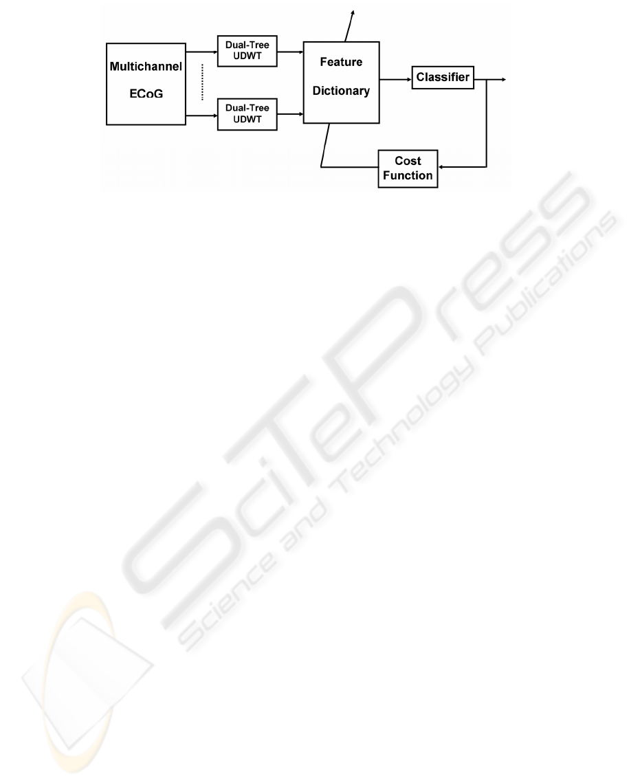
Figure 1: The block diagram of the proposed feature extraction and feature subset selection technique.

method weighs each electrode location for

classification and uses the correlation between

channels to increase the SNR of the extracted

features. Although the performance is increased with

CSP, it has been shown that this method requires a

number of electrodes to improve classification

accuracy and that it is very sensitive to electrode

montage. Furthermore, since it uses the variance of

each channel, this method does not account for the

spatiotemporal differences in distinct frequency

subbands. Recently, time-frequency methods have

been proposed as an alternative strategy for the

extraction of MI related patterns in BCI’s (Wang

2004, Ince2006 and Ince 2007). These methods

utilized the entire time-frequency plane of each

channel and integrate components with different

temporal and spectral characteristics. Promising

results were reported on well known data sets while

classifying multichannel EEG. One of the main

difficulties with these methods is once again dealing

with the high dimensionality of the data collected.

Furthermore, the adaptation to important patterns is

implemented either by only accounting for the

discrimination power of individual electrode

locations or simultaneous processing of a large

number of electrodes.

In this paper we tackle these problems by

implementing a spatially adapted time-frequency

plane feature extraction and classification strategy.

To our knowledge this is the first time that an

approach implements a joint processing of ECoG

features with different time and frequency resolution

coming from distinct cortical areas for classification

purposes. The algorithm proposed in this paper

requires no prior knowledge of relevant time-

frequency indices and related cortical areas. In

particular, as a first step, the proposed approach

implements a time-frequency plane feature

extraction strategy on each channel from

multichannel ECoG signals by using a dual-tree

undecimated wavelet packet transform (UDWT).

The dual-tree undecimated wavelet packet transform

forms a redundant, structured feature dictionary with

different t-f resolutions. In the next step, this

redundant dictionary is used for classification.

Rather than evaluating the individual discrimination

performance of each electrode or candidate feature,

the proposed approach selects a subset of features

from the redundant structured dictionary by

evaluating the classification performance of their

combination using a wrapper strategy. This enables

the algorithm to optimally select the most

discriminative features coming from different

cortical areas and/or time-frequency locations. A

block diagram summarizing the technical concept is

given in Figure 1. In order to evaluate the efficiency

of the proposed method we test it on the ECoG

dataset of BCI competition 2005.

The paper is organized as follows. In the next

section we describe the extraction of structural time-

frequency features with dual-tree undecimated

wavelet transform. In the following section we

discuss available feature selection procedures and

details of our proposed solutions. We describe the

multichannel ECoG data in section 4. Finally we

provide experimental results in section 5 and discuss

our findings in section 6.

2 FEATURE EXTRACTION

Let us describe our feature dictionary and explain

how it is computed from the wavelet-based dual-tree

structure. A schematic diagram of the dual tree is

shown in Figure 2. As indicated in the previous

sections, the ECoG can be divided into several

AN ECoG BASED BRAIN COMPUTER INTERFACE WITH SPATIALLY ADAPTED TIME-FREQUENCY

PATTERNS

133

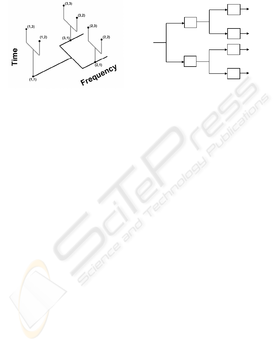
Figure 2: This dual tree uses 1-level in both planes. Each

node of the horizontal tree is a frequency subbands. Node

{1,1} represents unfiltered original signal, node{2,1}

represents low pass filtered signal and node {3,1} high

pass filtered. Each of these subbands is segmented in time

into 3 segments, as shown in the vertical tree. Segment

{1,1},{2,1} and {3,1} covers the whole subband, segment.

{1,2},{2,2} and {3,2} covers the first and segments with

time indices three the second half of it.

X[n]

H(z

)

G(z

)

H(z)

G(z)

H(z

)

G(z

)

[n]

Figure 3: The pyramidal undecimated wavelet tree.

frequency subbands with distinct and subject

depended characteristic. In order to extract

information from these rhythms, we examine

subbands of the ECoG signal by using an

undecimated wavelet transform. In each subband, a

second pyramidal tree is utilized to extract the time

varying characteristics of the subband.

2.1 Undecimated Wavelet Transform

Discrete Wavelet Transform (DWT) and its variants

have been extensively used in 1D and 2D signal

analysis (Vetterli 2001). However, the

downsampling operator at the outputs of each filter

produces a shift variant decomposition. In practice, a

shift in the signal is reflected by abrupt changes in

the extracted expansion coefficients or related

features. In (Unser 1995) the undecimated wavelet

transform is proposed to extract subband energy

features which are shift invariant. This is achieved

by removing the downsampling operation. The

output at any level of pyramidal filter bank is

computed by using an appropriate filter which is

derived by upsampling the basic filter.

A filter g(n) with a z-transform G(z) that satisfies the

quadrature mirror filter condition

() ( ) ( ) ( ) 1GzGz G zG z

−−

+− − = (1)

is used to construct the pyramidal filter bank (Figure

3). The high-pass filter h(n) is obtained by shifting

and modulating g(n). Specifically, the z transform of

h(n) is chosen as

() ( ).Hz zG z

−

=− (2)

The subsequent filters in the filter bank are then

generated by increasing the width of f(n) and g(n) at

every step, e.g.,

() ( )

Gz Gz

() ( )

HzHz

, (i=0,1,. . . . ., N). (3)

In the signal domain, the filter generation can be

expressed as

() []

↑

() []

hk h

↑

(4)

where the notation

m↑

[] denotes the up-sampling

operation by a factor of m.

The horizontal pyramidal tree of Fig.2 provides

subband decomposition of the ECoG signal. Next,

we segment the signal in each subband with

rectangular time windows. Such an approach will

extract the temporal information in each subband.

As in the frequency decomposition tree, every node

of the frequency tree is segmented into time

segments with a pyramidal tree structure. Each

parent time window covers a space as the union of

its children windows. In a given level, the length of

a window is equal to L/2

where L is the length of

signal and t denotes the level. The time segmentation

explained above forms the second branch (vertical)

of the double tree. After segmenting the signal in

time and frequency, we retain the energy of each

node of the dual-tree as a feature. By using a dual

tree structure we could calculate a rich library of

features describing the ECoG activities with several

BIOSIGNALS 2008 - International Conference on Bio-inspired Systems and Signal Processing

134

spectro-temporal resolutions. From now on we keep

the index information of the dual tree structure to be

used in the later stage for dimension reduction via

pruning.

To summarize this section the reader is referred to

the double tree structure in Fig. 2. Note that the dual

tree structure satisfies two conditions:

- For a given node in the frequency tree, the mother

band covers the same frequency band width (BW) as

the union of its children

( )

Mother Child Child

BW BW BW⊃∪ (5)

- This same condition is also satisfied along the time

axis. For a given node, the number of time samples

(TS) of the mother window is equal to that of the

union of its children.

( )

Mother Child Child

TS TS TS⊃∪ (6)

These two properties allow us to prune the tree

structure. When a particular feature index is

selected, one can remove those indices from the dual

tree structure that overlap in time and frequency

with the selected index. Let T be the number of

levels use to decompose the signal in time and F be

the number levels use to decompose the signal in the

frequency domain, there will be 2

(F+1)

-1 subbands

(including the original signal) and 2

(T+1)

-1 time

segments for each subband. This will make the total

number of potential features NF=(2

(F+1)

-1)(2

(T+1)

-1).

3 SUBSET SELECTION

Calculating the dual-tree features for each electrode

location forms a redundant feature dictionary. The

redundancy comes from the dual tree structure. As

explained in the previous section the dual tree has

total NF=(2

(F+1)

-1)(2

(T+1)

-1) features for each signal

where F is the total number of frequency levels and

T the total number of time levels. In a typical case,

T=3, F=4 and over 64 electrodes are used resulting

in a dictionary with around thirty thousand features.

In such a high dimensional space (NF=29760) the

classifier may easily go into over-learning and

provide a lower generalization capability.

Here, we incorporate the structural relationship

between features in the dictionary and use several

feature subset selection strategies to reduce the

dimensionality of the feature set. Since the features

are calculated in a tree structure, efficient algorithms

were proposed in the past for dimensionality

reduction. In (Saito 1996) a pruning approach was

proposed which utilizes the relationship between the

mother and children subspaces to decrease the

dimensionality of the feature set. In particular, each

tree is individually pruned from bottom to top by

maximizing a distance function. The resulting

features are sorted according to their discrimination

power and the top subset is used for classification.

Although such a filtering strategy with pruning will

provide significant dimension reduction by keeping

the most predictive features, it does not account for

the interrelations between features in the final

classification stage. Here, we reshape and combine

the pruning procedure for feature selection with a

wrapper strategy. In particular, we quantify the

efficiency of each feature subset by evaluating its

classification accuracy with a cost measure and we

use this cost to reformulate our dictionary via

pruning.

Four different types of methods are considered

for feature selection in this study. The structure in

Figure 1 is general representation of each of the four

methods. The left most box in Figure 1 is the rich

time-frequency feature dictionary. On the right end a

linear discriminant (LDA) is used both for

classification and extracting the relationship among

combinations of features. This output is fed to a cost

function to measure the discrimination power for

that combination of features. This measure will be

used to select the best among all other feature

combinations. Furthermore, depending on the

selected feature index, a pruning operation will be

implemented to reduce the dimensionality in the rich

feature dictionary.

In this particular study, the Fisher Discrimination

(FD) criterion is used as a cost function.

()

μμ

−

. (7)

The four different strategies mentioned above are:

Sequential forward feature selection (SFFS), SFFS

with pruning (SFFS-P), Cost function based pruning

and feature Selection (CFS), and CFS with principal

component analysis (PCA) post processing.

3.1 Sequential Forward Feature

Selection: SFFS

The SFFS is a wrapper strategy which selects a

subset of features one by one. A cost function is

used on classifier output to measure the efficiency of

each feature. By using LDA, the feature vectors are

projected on a one dimensional space. Then the FD

criterion was used to estimate the efficiency of the

projection. After this search is done over all feature

vectors, the best feature index is selected by

AN ECoG BASED BRAIN COMPUTER INTERFACE WITH SPATIALLY ADAPTED TIME-FREQUENCY

PATTERNS

135

(a)

(b)

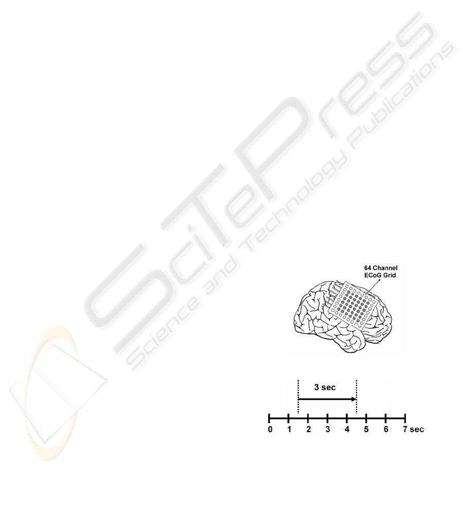
Figure 4: The 8x8 electrode grid was placed on the right

hemisphere over the motor cortex (Modified from Lal

2005). For surface Laplacian derivation only marke

electrodes are used. (b) The timing diagram of the

experimental paradigm. The go cue for motor imagery is

given at second one. A three second time window starting

after 500ms of go cue is used to classify ECoG data.

comparing the cost values of each feature vector. In

the next step the feature vector which will do the

best in combination with the first selected ones is

identified by searching over the remaining feature

vectors. This procedure is run until a desired number

of features is reached. Note that SFFS uses all the

boxes and connections in Figure 1 except for the

feedback from the cost function to the dictionary.

Since no dimension reduction is implemented on the

entire feature space, this approach has high

computational complexity.

3.2 SFFS with Pruning: SFFS-P

The SFFS-P is also a wrapper strategy with an

additional pruning module for dimension reduction.

Once a feature index is selected, the corresponding

frequency tree and time tree indexes are calculated

on the dual-tree. Then the nodes that overlap with

the selected feature index in time and frequency are

removed. Next, the feature which will do best in

combination with the first selected feature is

identified by searching the pruned dictionary. In

other words, the dictionary is pruned based on the

last selected feature. This procedure is run until the

desired number of features is reached. Therefore, the

only difference between SFFS and SFFS-P is that

pruning is done on the dictionary based on the

selected features. This provides a fast decrease in the

number of candidate features and complexity is

much smaller than SFFS.

3.3 Cost Function based Pruning and

Feature Selection (CFS)

The CFS is a filtering approach that uses the

structure in the feature dictionary for pruning. After

finalizing the pruning procedure for each electrode

location, it uses a cost function to rank the features.

In particular, it uses the FD criterion to rank the

features. It does not use either the LDA or the

feedback path in Figure 1. Instead, using the FD

measure, a cost value is computed for each node on

the double tree individually. Then a pruning

algorithm is run on the double tree by keeping the

nodes with maximum discrimination. Once a node is

selected all nodes overlapping with the selected one

are removed. This procedure is iterated until no

pruning can be implemented. After pruning the dual-

trees for each electrode location, the resulting

feature set is sorted according to their corresponding

discrimination power and input to the classifier. In

this way the most predictive features were entered to

the classification module. Since no feedback is used

from the classifier, the CFS has lower computational

complexity than the other two methods.

The CFS method works as a filter on the electrodes

by only keeping those indices with maximum

discrimination power. However, since features are

evaluated according to their discrimination power

individually, such a method does not account for the

correlations between features. In (Ince 2006 and

Ince 2007) PCA analysis is performed on a subset of

top sorted features to obtain a decorrelated feature

set. The PCA post processed features are sorted

according to their corresponding eigenvalues in

decreasing order and used in classification. Here we

will also use the PCA as a post processing step with

the CFS to obtain a deccorelated feature set. We will

refer this method as CFS-PCA.

4 MULTICHANNEL ECoG DATA

In order to evaluate the performance of the proposed

method we used the multichannel ECoG (Lal 2005)

dataset of BCI competition 2005

(ida.first.fraunhofer.de/projects/bci/competition_iii/)

During the BCI experiment, a subject had to perform

imagined movements of either the left small finger

or the tongue. The ECoG data was recorded using an

8x8 ECoG platinum electrode grid which was placed

on the contralateral (right) motor cortex as shown in

Figure 4. All recordings were performed with a

sampling rate of 1000Hz. Every trial consisted of

either an imagined tongue or an imagined finger

movement and was recorded for 3 seconds duration.

To avoid visually evoked potentials being reflected

BIOSIGNALS 2008 - International Conference on Bio-inspired Systems and Signal Processing

136

1 8

57 64

(a) (b)

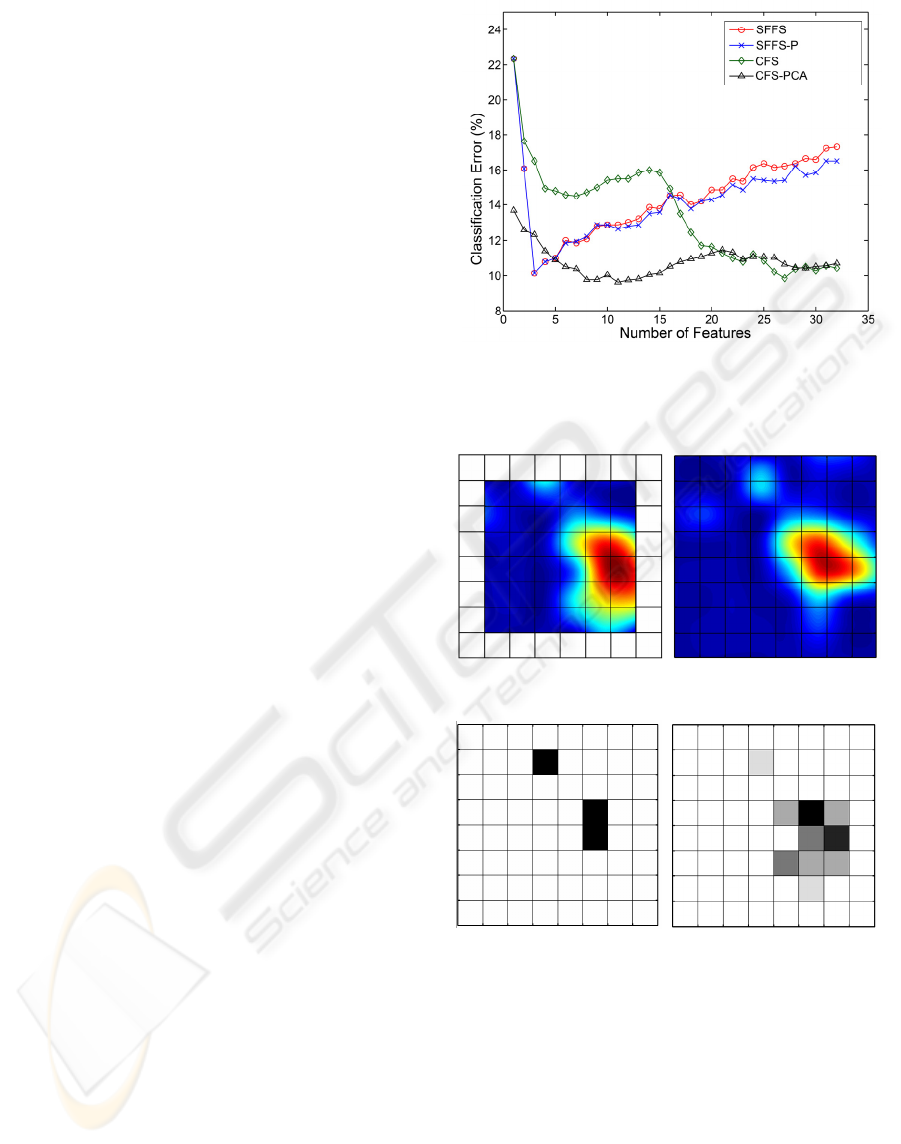
Figure 6: Discriminant cortical areas (a) Laplacian (b)

Monopolar. The number of selected features fro

different electrode locations in Laplacian derivation fo

SFFS-P (c) and for CSF(d) are given. The darker areas

indicate a higher number of features are selected fro

these regions. Note that SFFS-P provides a balance

feature distribution. The CSF selected most of 27 features

from the same region.

Figure 5: The cross validation error curves for the

different methods in the training data.

by the data, the recording intervals started 0.5

seconds after the visual cue had ended. Each channel

was filtered with a low pass filter in 0-120Hz band.

The filtered data was down sampled by a factor 4 to

250Hz. Each trial was expanded from 750 samples

into 768 samples by symmetric extension on the

right side to enable segmentation in a pyramidal tree

structure. Besides monopolar data, we also consider

ECoG data that is processed using a surface

Laplacian derivation. More specifically, each

electrode data is subtracted from the weighted

average of the surrounding 6 electrodes. The

electrodes on the border are eliminated from the

analysis resulting in a total of 36 electrodes (See

Figure 4). For monopolar data all 64 electrodes were

used for analysis. We used 278 trials for training and

100 trials for testing. The training and test data were

recorded from the same subject and with the same

task, but on two different days with about 1 week in

between.

5 RESULTS

To extract the dual tree features we select T=3 and

F=4. For a 125 Hz bandwidth, the frequency tree

provided around 8Hz resolution at the finest level.

Along the time axis, the time resolution was 375ms.

The 12 tap Daubechies filter (db6) was used in

constructing the frequency tree of the UDWT. In

order to learn the most discriminant time-frequency

indices and the corresponding cortical areas we

utilized a 10 times 10 fold cross validation in the

training dataset. The optimal feature number at

which the classification error is minimal is selected

from the averaged cross validation error curves.

Then, the learned feature indices are used in testing

the classifier on the test set. The results obtained

with the different methods are presented in Table.1.

We note that the SFFS and SFFS-P provided the

highest classification accuracy with only three

features on the test set using the Laplacian

derivation. Although a lower error rate was achieved

by CFS with the training data, interestingly, the

testing error rate of the CFS was higher than those of

the other methods. We also note that a large number

of features were used by CFS to achieve 9.9% error

rate in the training set. In contrast, the SFFS and

SFFS-P algorithms used only 3 features to achieve

the minimum 10.2% error rate. The cross validation

error curves versus the number of features are given

in Figure 5. Since the results using Laplacian

derivation outperformed those obtained with

monopolar data, only the results corresponding to

the former are provided.

As can be seen clearly from these curves, SFFS and

SFFS-P select the best combination of features and

achieve the minimal error with only three features.

AN ECoG BASED BRAIN COMPUTER INTERFACE WITH SPATIALLY ADAPTED TIME-FREQUENCY

PATTERNS

137

Table 1: The cross validation (CV) and test error rates of different methods and related number of features (NoF) used for

final classification.

Training Test

Method CV Error (%) NoF Error (%)

SFFS 10.2 3 7

SFFS-P 10.2 3 7

CSF 9.9 27 18

Laplacian

CSF-PCA 9.6 11 8

SFFS 12.6 3 20

SFFS-P 10.3 4 9

CSF 11.7 22 12

Monopolar

CSF-PCA 11.2 14 8

Furthermore, using the structure of the feature

dictionary, SFFS-P achieves this result with reduced

complexity due to pruning. The pruning process

provides a dimension reduction and feature

decorrelation. CFS, on the other hand, achieves the

minimal error using a large number of features. The

interactions among the selected features cannot be

taken into account with this approach. In addition

the correlated neighbor areas may result in a

duplication of information in the sorted features. In

order to decorrelate the features a Principal

Component Analysis (PCA) was employed on the

CFS ordered features. This post processing step

provided lower error rates than those achieved by

CFS alone. The test error rate was 8% for the PCA

post processed features. It should be noted here that

CFS-PCA produced comparable results with those

of SFFS and SFFS-P. However one should note that

PCA induces an additional complexity. This method

requires all 32 features to be extracted from ECoG

which leads to a much higher computational

complexity compared to three features selected by

SFFS and SFFS-P.

Since the testing data was recorded on another date,

the variability in the ECoG signal is expected. The

results obtained indicate that the CFS algorithm is

very sensitive to this type of variability. Although

the cross validation error in the training set was low,

the testing error rate was much higher compared to

other methods. We believe that the correlated

activity across cortical areas is an important reason

why CFS selects the same information repeatedly.

Since the SFFS and SFFS-P have the advantage of

examining the interactions between different cortical

areas and t-f locations, these subset selection

algorithms can form a more effective subset of

features for classification. In order to support our

hypothesis we show the discriminatory cortical maps

of monopolar and Laplacian derivations in Figure 6.

In order to generate these images we used the most

discriminant feature of each electrode location and

produced an image over the 8x8 grid to present the

distribution of the most discriminative locations.

Furthermore, we mark the electrode locations

selected by SFFS, SFFS-P, and CFS for

classification. After inspecting Figure 6 (a) and (b)

we noticed that a large number of neighbor electrode

locations carry discriminant information. The CFS

method used a large number of electrodes from this

region for classification. In contrast, the SFFS and

SFFS-P methods selected another cortical area from

upper side of the grid. Even though this electrode

location does not seem to be very discriminative, it

played a key role in achieving a lower classification

rate on the validation data.

Since only three features are used by SFFS and

SFFS-P, they are more robust to intra-subject

variability of ECoG signals. Note also that the error

rate in monopolar derivation is much higher than

that of the Laplacian derivation. We observed large

DC changes in ECoG signals in the test data set.

Since the Laplacian derivation provides a

differential operator, large baseline wanders

affecting many electrodes are eliminated in this

setup. However, for the monopolar recordings the

features are very sensitive to this type of changes.

Note also that the validation accuracy of SFFS

and SFFS-P in the test set is higher than the cross

validation accuracy. One of the underlying reasons

could be that the subject can control his/her brain

patterns with a higher accuracy with the increasing

number of trials. In addition the SNR of the signals

might have improved over time due to tissue

electrode interaction.

Finally, we compared our proposed method’s

test result with those of achieved at the BCI

competition in 2005 using the same ECoG data. The

classification accuracies and methods used in each

method are presented in Table 2. Our method

achieved the best result of 7% error with both SFFS

BIOSIGNALS 2008 - International Conference on Bio-inspired Systems and Signal Processing

138

Table 2: The comparison of the proposed method with the

best three methods from the BCI 2005 competition.

Features Used Classifier Error (%)

UDWT based

subband energies

LDA 7

Common Spatial

Subspace

Decomposition

Linear SVM 9

ICA combined with

spectral power and

AR coefficients

Regularized

logistic

regression

Spectral power of

manually selected

channels

Logistic

regression

and SFFS-P methods. We note that our proposed

approach has outperformed both CSP and AR model

based techniques.

6 CONCLUSIONS

In this paper we proposed a new feature extraction

and classification strategy for multi-channel ECoG

recordings in a BCI task. Rather than using

predefined frequency indices or manually selecting

cortical areas, the algorithm implemented an

automatic feature extraction and subset selection

procedure over a redundant time-frequency feature

dictionary. This feature dictionary was obtained by

decomposing the ECoG signals into subbands with

an undecimated wavelet transform and then

segmenting each subbband in time successively. By

combining a wrapper strategy with dictionary

pruning, the method achieved 93% classification

accuracy using only three features. The results we

obtained show that the proposed method is a good

candidate for the construction of an ECoG based

invasive BCI system with very low computational

complexity and high classification accuracy.

REFERENCES

Ince N. F., Tewfik A., Arica S., 2007, “Extraction subject-

specific motor imagery time-frequency patterns for

single trial EEG classification”, Comp. Biol. Med.

Elsevier.

Ince N. F., Arica S., Tewfik A., 2007, “Classification of

single trial motor imagery EEG recordings by using

subject adapted non-dyadic arbitrary time-frequency

tilings,” J. Neural Eng. 3, 235-244.

Lal Thomas N., et.al., 2005, Methods Towards Invasive

Human Brain Computer Interfaces. Advances in

Neural Information Processing Systems (NIPS17, 737-

744. (Eds.) Saul, L. K., Y. Weiss, L. Bottou, MIT Press,

Cambridge, MA, USA).

Leuthardt E. C. , Schalk G., Wolpaw J. R., Ojemann J. G.

and Moran D. W., 2004, A brain–computer interface

using electrocorticographic signals in humans, Journal

of Neural Engineering, pp. 63–71.

Pfurtscheller G., Neuper C., 2001. Motor Imagery and

Direct Brain-Computer Interface. Proceedings of

IEEE, vol.89, pp. 1123-1134.

Prezenger M., Pfurtscheller G., 1999. Frequency

component selection for an EEG-based brain computer

interface. IEEE Trans. on Rehabil. Eng. 7, pp. 413-

419.

Ramoser H., Müller-Gerking J., and Pfurtscheller G.,

2000. Optimal spatial filtering of single trial EEG

during imagined hand movement. IEEE Trans. Rehab.

Eng., vol. 8, no. 4, pp. 441–446.

Saito N. et al., 2002, Discriminant feature extraction using

empirical probability density and a local basis library,

Pattern Recognition, vol.35, pp. 1842-1852.

Schlögl A., Flotzinger D., Pfurtscheller G., 1997. Adaptive

autoregressive modeling used for single trial EEG

classification. Biomed. Technik,42, pp. 162-167.

Unser M., 1995. Texture classification and segmentation

using wavelet frames. IEEE Trans. Image Proc., pp.

1549–60, Vol.4(11), Nov.

Vetterli M., 2001. Wavelets, approximation, and

compression,'' IEEE Signal Proc. Magazine, pp. 59–

73, Sept..

Wang T., and B. He, 2004. Classifying EEG-based motor

imagery tasks by means of time–frequency

synthesized spatial patterns. Clin. Neuro. vol.115, pp.

2744–2753.

Wolpaw J. R., et.al., 2000. Brain-Computer Interface

Technology: A review of the first international

meeting, IEEE Trans. On Rehab. Eng. 8 164-73.

AN ECoG BASED BRAIN COMPUTER INTERFACE WITH SPATIALLY ADAPTED TIME-FREQUENCY

PATTERNS

139