
CLUSTERED CELL SEGMENTATION
Based on Iterative Voting and the Level Set Method
Arjan Kuijper
Johann Radon Institute for Computational and Applied Mathematics, Altenberger Strasse 69, Linz, Austria
Yayun Zhou
Mathematical Engineering - CT PP 2, Siemens AG, Otto-Hahn-Ring 6, Munich, Germany
Bettina Heise
Dept. of Knowledge-Based Mathematical Systems, Johannes Kepler University, Altenberger Strasse 69, Linz, Austria
Keywords:
Cell segmentation, voting methods, level sets, parameter setting, evaluation.
Abstract:
In this paper we deal with images in which the cells cluster together and the boundaries of the cells are
ambiguous. Combining the outcome of an automatic point detector with the multiphase level set method, the
centre of each cell is detected and used as the ”seed”, in other words, the initial condition for level set method.
Then by choosing appropriate level set equation, the fronts of the seeds propagate and finally stop near the
boundary of the cells. This method solves the cluster problem and can distinguish individual cells properly,
therefore it is useful in cell segmentation. By using this method, we can count the number of the cells and
calculate the area of each cell. Furthermore, this information can be used to get the histogram of the cell
image.
1 INTRODUCTION
Cell segmentation is a popular topic in image analy-
sis. Typically, the population of cells in one image is
large. If we want to count the number of the cells, or
study the property of certain cell, cell segmentation is
necessary and important. In general, a reliable seg-
mentation is hard because images are noisy (both ran-
dom and speckle noise). Sometimes many cells will
cluster together and even overlap in the sample. This
complicated situation makes the problem more chal-
lenging and interesting. There is a wide variety of
approaches focusing on different segmentation prob-
lems.
Nowadays, one of the popular approaches is the
active contour model, or snakes, (Kass et al., 1988).
The basic idea in active contour models (or snakes)
is to evolve a curve, subject to constraints from a
given image u
0
, in order to detect objects in that im-
age. Usually, the model contains an edge detector,
which depends on the gradient of the image u
0
. The
initial curve is around the object to be detected, then
the curve moves in the normal dimension to itself and
ideally stops at the boundary of the object. The main
drawbacks of the original snakes are their sensitiv-
ity to initial conditions and the difficulties associated
with topological transformations.
Another famous model in image segmentation
(Mumford and Shah, 1989) proposes a minimisation
problem. The minimiser for the functionals is the op-
timal piecewise smooth approximation u for the given
image u
0
. In practise, solving the Mumford and Shah
model is not an easy job, because the functional in-
volves an unknown set C of lower dimension and usu-
ally the problem is not convex.
1.1 The Level Set Method in Image
Segmentation
In this work we will focus on the level set method.
The level set method is a numerical and theoretical
tool for propagating interfaces (Osher and Sethian,
1988; Sethian, 1999), and has become a more and
more popular theoretical and numerical framework
within image processing, fluid mechanics, graphics,
computer vision, etc. The level set method is basi-
307
Kuijper A., Zhou Y. and Heise B. (2008).
CLUSTERED CELL SEGMENTATION - Based on Iterative Voting and the Level Set Method.
In Proceedings of the Third International Conference on Computer Vision Theory and Applications, pages 307-314
DOI: 10.5220/0001070603070314
Copyright
c
SciTePress
cally used for tracking moving fronts by considering
the front as the zero level set of an embedded function,
called the level set function. In image processing, it is
used for propagating curves in 2D or surfaces in 3D.
The applications of the level set method cover most
fields in image processing, such as noise removal, im-
age inpainting, image segmentation and reconstruc-
tion (Osher and Paragios, 2003).
In image segmentation, the level set method has
some advantages compared to the active contour
model. The level set method conquers the difficul-
ties of topological transformations. The level set ap-
proach is able to handle complex topological changes
automatically.
For images with clustered cells, the traditional
level set method is not suitable for segmenting in-
dividual cells. In this work, we will use a method
designed especially for these kind of images. The
main idea of this method is using an iterative voting
method to detect the centre of each cell (Yang et al.,
2004). The detected centre is used to define the ini-
tial condition for the level set method. A sequence of
level set functions are set up for each cell (Solorzano
et al., 2001). Combining with the initial condition, the
PDEs for each cell can be solved numerically. This
method is tested on different cell images, with both
regular and irregular patterns, and overlapping cells.
The performance is stable. As long as the cells are
distinguishable by human eyes, the algorithm can seg-
ment individual cells properly.
Full details on the methodology and comparisons
with related methods can found in our technical report
(Zhou et al., 2007).
2 SEED DETECTION
The first step for this segmentation method is detect-
ing the centre of cells. Since the detected centre will
be used as the initial condition (”seed”) for the level
set method, this step is very important for the per-
formance of the whole method. The number of de-
tected seeds determines the number of cells which can
be detected. If there are some cells without seeds, it
means that these cells will not be counted in as candi-
dates. If there are two seeds in one cell, it may cause
over-segmentation (a cell is divided into two cells).
In brief, the accuracy of the first step will affect the
performance of the level set methods.
2.1 Iterative Voting
Since the shape of cells has some important proper-
ties, such as symmetry, continuity and closure, we
apply an iterative voting method using oriented ker-
nels to detect the candidate position for the centre of
the cell (Yang et al., 2004). The basic idea of this al-
gorithm is also a voting method, but instead of trans-
forming into other parameter spaces like the Hough
Transform, it defines a series of kernels that vote it-
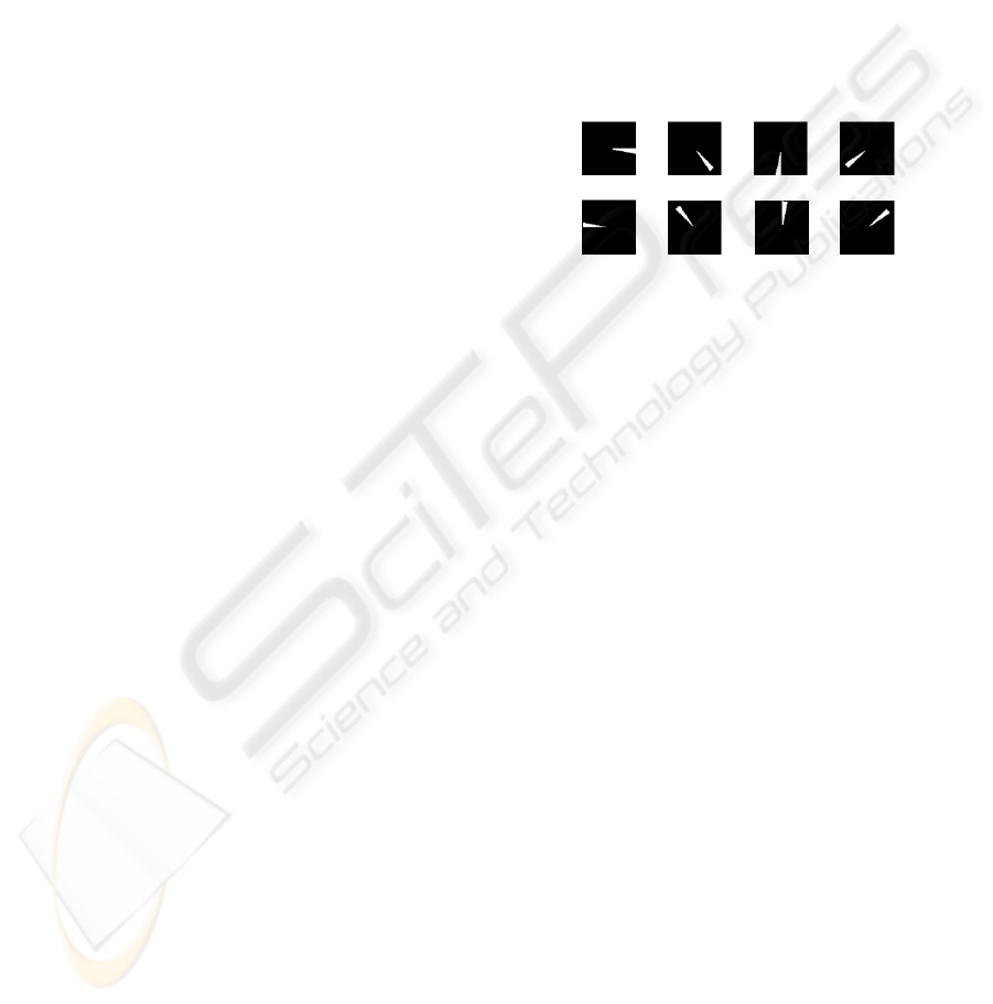
eratively along radial direction. The kernel is cone-
shaped, as Fig. 1 shows. Applying this kernel along
the gradient direction, at each iteration and each grid
location, the orientation of the kernel is updated. The
shape of the kernel is also refined and focused as the
iterative process continues. Finally, the point of inter-
est is selected by certain threshold.
Figure 1: Shape of Kernel used in the Method.
Let I(x,y) be the original image, α(x,y) be the vot-
ing direction where α(x,y) := (cosθ(x,y),sinθ(x,y)),
(r
min
,r
max
) be the radial range, V be the voted image,
and A be the voting area defined by
A(x,y;r
min
,r
max
,∆) := {(x ±r cos θ, y ±r sin φ),
|r
min
< r < r
max
,θ(x,y) −∆ ≤ φ ≤ θ(x,y) + ∆}.
(1)
Let G(x,y; σ,α,A) be a 2D Gaussian kernel
with variance σ, masked by the local voting area
A(x,y;r
min
,r
max
,∆) and oriented in the voting direc-
tion α(x,y). Then the iterative voting algorithm con-
tains following seven steps; for the detailed imple-
mentation see (Yang et al., 2004):
1. Initialise the parameters: r
min
,r
max
,∆
max
and a se-
quence ∆
max
= ∆
N
> ∆
N−1
> . . . > ∆
0
= 0, set
n := N, where N is the number of iterations, ∆
n
=
∆
max
, fix a low gradient threshold Γ
g
and a ker-
nel variance σ depending on the expected scale of
salient features.
2. Initialise the saliency feature image: Define the
feature image F(x,y) to be the local external force
at each pixel of the original image. The exter-
nal force is often set to the gradient magnitude or
maximum curvature, depending upon the type of
saliency grouping and the presence of local fea-
ture boundaries.
3. Initialise voting direction and magnitude: Com-
pute ∇(I), its magnitudek∇(I)k, define a pixel
VISAPP 2008 - International Conference on Computer Vision Theory and Applications
308
subset S := {(x, y)|k∇(I)k > Γ
g
}, for each pixel
(x,y) ∈ S, let the voting direction be
α(x,y) := −
(I
x
(x,y),I
y
(x,y))
k∇(I)k
. (2)
4. Compute the votes: V (x,y;r
min
,r
max
,∆) = 0. For
all pixels (x,y) ∈ S, update the vote image:
V (x, y; r
min
,r
max
,∆) = V (x, y; r
min
,r
max
,∆)
+
∑
(u,v)∈A
F(x −
w
2
+ u,y −
h
2
+ v)G(u,v; σ,α,A),
(3)
where w = max(u) and h = max(v) are the maxi-
mum dimensions of the voting area.
5. Update the voting direction: For grid points
(x,y) ∈ S, revise the voting direction:
(u
∗
,v
∗
) = arg max
(u,v)∈A(x,y;r
min
,r
max
,∆)
V (u,v; r
min
,r
max
,∆).
(4)
Let d
x
= u
∗
−x,d
y
= v
∗
−y, and α(x, y) =
(d
x
,d
y
)
√
d
2
x
+d
2
y
.
6. Refine the angular range: Let n := n −1, repeat
steps 4 −6 until n = 0.
7. Localise centres of mass: by threshold
{(x,y)|V (x, y; r
min
,r
max
,∆) > Γ
v
}, (5)
This gives a binary image with interested points.
These points show the locations of the cell centres.
2.2 Results for Seed Detection
The algorithm is tested on a data base with differ-
ent types of images. We selected six typical images,
showing three types of cell clustering for which re-
sults can be verified by human observers. The com-
plete data base also contains images with completely
overlapping and out-of-focus cells. In these cases, hu-
man observers cannot distinguish individual cells.
By adjusting the parameters r
min
, r
max
, nsectors
and thresh, the seed for each cell is detected accu-
rately. The adjustment of parameters is discussed in
the following subsection. Usually, four or five itera-
tions are enough to determine the location of seeds, so
this algorithm is more efficient than the Hough Trans-
form and the performance of seed detecting is satis-
factory. The following figures show some examples
of seed detection on the different types.
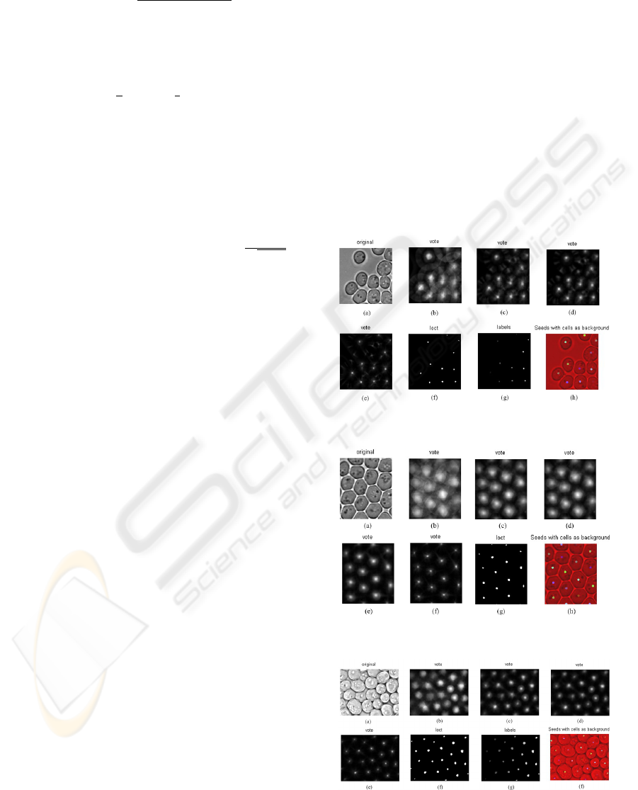
In Fig. 2, the sub-figure (a) is the original im-
age, in which the cells are scattered and parts of the
cells are close to each other. The following four sub-
figures show the procedure of applying iterative vot-
ing method. After the iterative voting procedure, a
threshold is applied in order to get the binary image
named ”loct” (sub-figure (e)), these white spots in the
sub-figure ”loct” are the location of the seeds. The
seeds are marked with different numbers and the re-
sult is shown with different grey levels, yielding the
sub-figure (f) named ”label”. The last one shows the
seed locations at the background of original image 1n
order to check the relative location. From that we can
see the seed locations are approximately in the middle
of each cell, as expected.
In Fig. 3, the shape of the cells is not exactly el-
liptic and all the cells are clustered together. Different
from Fig. 2, this voting procedure needs five steps.
But after all, all seeds are detected and located in the
middle of each cell, which can be seen from the last
sub-figure.
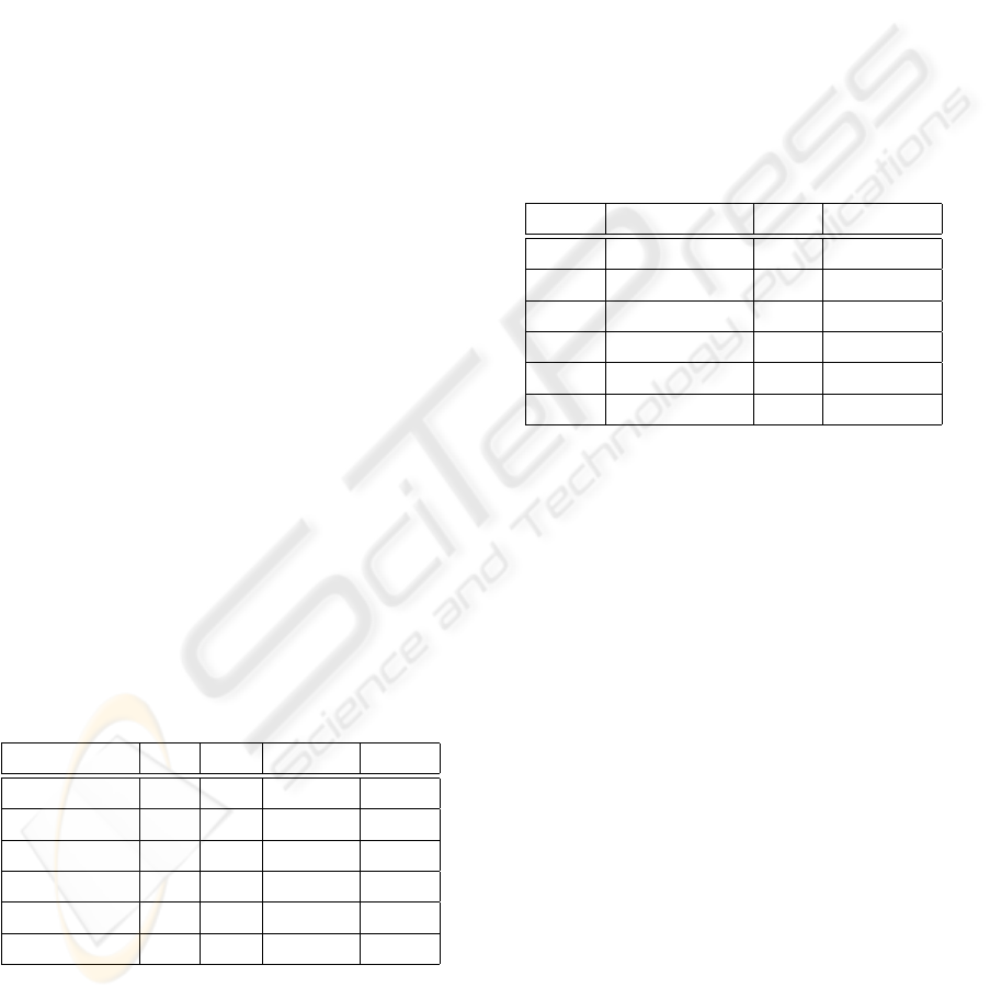
In Fig. 4, the test image is more difficult since
some of the cells even overlap each other and the sizes
of the cells are different. This algorithm still can de-
tect all the cells and show the location of each cell.
Figure 2: Seed Detection Result for image 1.
Figure 3: Seed Detection Result for image 2.
Figure 4: Seed Detection Result for image 4.
CLUSTERED CELL SEGMENTATION - Based on Iterative Voting and the Level Set Method
309
2.3 Parameter Setting and Operation
Time
There are four important parameters in seed detection
part, they are r
max
, r
min
, nsectors and thresh. The
parameters r
max
and r
min
determine the voting area,
nsector determines the number of iteration; thresh de-
termines the value of threshold applied after the vot-
ing procedure. Those parameters are set up according
to the following rules:
• The r
max
usually equals to the radius of the cell.
If the radii of the cells are different, then choosing
the maximum radius is acceptable.
• The value of the r
min
is used to avoid noise effects,
usually it equals 4 or 5.
• The number of iteration n
iter
:= nsectors/8−1, so
the value of nsector should be multiples of 8. For
most cases, 4 iterations are enough to determine
the location of seeds. If the shape of cell is not
regular, then more iteration steps are needed.
• The value of the threshold can vary from 1.0 to
around 8.0, it depends on the noise properties of
the images. The key idea to determine the value
is to set the number of false positives as small as
possible.
Adjusting parameter needs some experience, but
for certain type of cells, the parameters are fixed.
Generally speaking, this program is stable and easy to
implement. The result is especially good for clustered
cells, because the cells have radial symmetric prop-
erties but the background doesn’t have this property.
Table 1 shows some example of parameters setting,
from which we can see some of the rules discussed
above.
Table 1: Parameter Setting for Seeds Detection Part.
Image Name r
min
r
max
nsectors thresh
image 1 5 19 40 6
image 2 5 30 48 4
image 3 5 30 40 2
image 4 4 25 40 2.5
image 5 4 25 40 4
image 6 4 25 40 2.5
This method is relatively fast since the iteration
number is not large. As we expect, the operation time
depends on the image size and the voting area.
From the Table 2, we can see that the larger the im-
age size is, the more time is needed for the procedure.
Iteration number is also an important factor influenc-
ing the operation time. Images 1 and 2 have similar
size, but the operation time for image 2 is much larger
than image 1, because the image 2 needs five itera-
tions while image 1 only needs four iterations.
Furthermore, the parameters r
min
and r
max
have in-
fluence to operation time as well, because these two
parameters determine the voting area. The larger the
voting area is, the more operation time is needed. We
can see the effect from the Table 1 and the Table 2.
The image size of ”image 4” is larger than ”image
3”, and the iteration numbers for both images are the
same, but the operation time of ”image 4” is less than
”image 3”. The reason is that the voting area of ”im-
age 4” is smaller than ”image 3”.
Table 2: Operation Time for Seeds Detection Part.
Image Size of Image ] iter Time (sec)
1 138 ×130 4 7.81
2 140 ×120 5 33.83
3 150 ×150 4 29.11
4 176 ×139 4 23.04
5 200 ×200 4 37.54
6 256 ×256 4 58.74
3 LEVEL SET METHOD FOR
CLUSTERED CELL IMAGE
After detecting the centre of each cell, we already
know the number of cells. The next step is to de-
tect each candidate cell. This part contains three steps
(Malladi and Sethian, 1995; Solorzano et al., 2001),
each step refers to a level set equation.
The initial condition for the level set equation is
inside the cell, so the first equation, which describes
the interface evolution, should grow outwards. The
model contains a stopping criterion which will stop
the evolution when it approaches the edge of detected
cells. After this procedure, the interface will stop near
the internal boundary of cells. This is essential, since
the level sets may not merge.
The second step is to set up another level set equa-
tion removing the boundary detect term to let the in-
terface keep growing. The only constraint for the sec-
ond step is that the growing fronts can’t penetrate each
other. The second step is only allowed for finite steps
to ensure the front exceed the cell boundary.
The last step is to move the interface inwards
again until it finds the external cell boundary.
VISAPP 2008 - International Conference on Computer Vision Theory and Applications
310

3.1 Initial Expansion
Motivated by the traditional level set model, the fol-
lowing level set equation is defined (Solorzano et al.,
2001):
φ
t
+ g ·(1 −εκ) ·|∇φ|−β∇g ·∇φ = 0, (6)
where g = e
−α|∇(G∗I
0
(x))|
, α > 0, G ∗I
0
(x) is the con-
volution of the original image I
0
(x) with a Gaussian
function G. The speed function F = g ·(1 −εκ) con-
tains an inflationary term (+1), which determines the
direction of evolution to be outward. The curvature
term (εκ) regularises the surface by accelerating the
movement of those parts of surface behind the aver-
age of the front and slowing down the advanced parts
of flow. The parameter ε determines the strength of
regularization, if ε is large, it will smooth out front
irregularities. For extreme cases, the final front will
become a circle. If ε is small, the front will main-
tain sharp corners. In practise, an intermediate value
of ε is chosen that allows the front to have concav-
ities (concavities are possible for cell border), while
small gaps and noise are smoothed. The effect of g is
to speed up the flow in those areas where the image
gradient is low and slowing down where the image
gradient is high. Because of this term, the front slows
down almost to stop when it reaches the internal cell
boundary. The parameter α determines the sensitivity
of the flow to the gradient. The extra term β∇g ·∇φ is
a parabolic term that enhances the edge effect.
In this step, there is another restriction condition
for the equation: The growing front may not invade
(and merge with) other cells’ region when seed grows.
By using this level set equation, the internal boundary
of the cells is detected.
3.2 Free Expansion
The initial expansion level set function usually causes
underestimation of cell area due to the thick bound-
ary. So a second and third step are added to compen-
sate the result. The second step is the free expansion,
in which the front is allowed to expand freely and the
speed of evolution doesn’t rely on the gradient of orig-
inal image. The level set equation is simply defined
as below:
φ
t
+ |∇φ|= 0. (7)
Similar as the first step, the growing fronts may
not penetrate each other when the front expands. This
expansion only needs a number of steps to ensure that
all the fronts move beyond the external boundary of
cells. The number of iteration depends on the thick-
ness of the cell boundary.
3.3 Surface Wrapping
After the free expansion step, the fronts are located
outside the cells’ boundary. The last step is to move
the front inwards to get the exact location of the exter-
nal cell boundary. So the speed function F = g ·(−1−
εκ) contains an shrinking term (−1), which deter-
mines the direction of evolution to be inward. Similar
to the initial expansion flow, g = e
−α|∇(G∗I
0
(x))|
, α >
0, G ∗I
0
(x) is the convolution of the original image
I
0
(x) with a Gaussian function G. The effect of this
term is to detect the external boundary of the cells.
The parameter α can be different value from the initial
expansion. In short, the level set equation is defined
as:
φ
t
+ g ·(−1 −εκ)|∇φ| = 0. (8)
3.4 Numerical Implementation
First, we define some notations which will be used
in the numerical implementation. D
+x
is the forward
difference approximation for the spatial derivative u
x
.
Similarly, D
−x
is the backward difference approxima-
tion and D
0x
is the central difference approximation,
which are defined respectively as follows:
D
+x
u ≡
u(x + h,t) −u(x,t)
h
, (9a)
D
−x
u ≡
u(x,t) −u(x −h,t)
h
, (9b)
D
0x
u ≡
u(x + h,t) −u(x −h,t)
2h
. (9c)
The operators ∇
+
and ∇
−
are calculated as follows:
∇
+
=
[max(D
−x
i j
,0)
2
+ min(D
+x
i j
,0)
2
+
max(D
−y
i j
,0)
2
+ min(D
+y
i j
,0)
2
]
1/2
,
(10)
∇
−
=
[max(D
+x
i j
,0)
2
+ min(D
−x
i j
,0)
2
+
max(D
+y
i j
,0)
2
+ min(D
−y
i j
,0)
2
]
1/2
,
(11)
In general, the numerical implementation for the level
set equations defined above is followed the algorithm
introduced in (Sethian, 1999). In brief, it can be de-
noted as the following equation:
φ
n+1
i j
= φ
n
i j
+ ∆tR (12)
with
R =
−[max(F
0i j
,0)∇
+
+ min(F
0i j
,0)∇
−
]
−
(
[max(u
n
i j
,0)D
−x
i j
+ min(u
n
i j
)D
+x
i j
+max(v
n
i j
,0)D
−y
i j
+ min(v
n
i j
)D
+y
i j
)
+[εK
n
i, j
((D
0x
i j
)
2
+ (D
0y
i j
)
2
)
1/2
]
.
(13)
CLUSTERED CELL SEGMENTATION - Based on Iterative Voting and the Level Set Method
311

For the initial expansion level set function Eq. (6),
F
0
refers to g, (u,v) refers to −β∇g, and K refers to
g ·κ in Eq. (6).
For the free expansion level set function Eq. (7),
F
0
≡ 1 and the other terms are eliminated. So the Eq.
(12) is reduced to:
φ
n+1
i j
= φ
n
i j
−∆t ·∇
+
, (14)
For the surface wrapping level set function Eq. (8), F
0
refers to −g, which is negative, K refers to g ·κ in Eq.
(8) and (u, v) ≡ 0. So the equation can be rewritten
as:
φ
n+1
i j
= φ
n
i j
+∆t[−g·∇
−
+(εK
n
i, j
((D
0x
i j
)
2
+(D
0y
i j
)
2
)
1/2
)].
(15)
Another restriction condition for the equation is that
the front may not invade other cells’ region when
the seed grows. But in the iteration procedure, ev-
ery front is moving independently from other fronts.
To avoid the penetration phenomenon, in every it-
eration step, the outcome is considered as a trial
function. By comparing with other fronts in pre-
vious steps using the following standard: φ
i
m+1
=
max{φ
i
m+1(trial)
,−φ
j
m
}, i ≤ j ≤ n, i 6= j, the final
movement of the front is determined.
For the three level set equations, a reinitialisation
phase is necessary. The purpose of reinitialisation
is to keep the evolving level set function close to a
signed distance function during the evolution. It is a
numerical remedy for maintaining stable curve evolu-
tion (Sussman and Fatemi, 1999). The reinitialisation
step is to solve the following evolution equation:
ψ
τ
= sign(φ(t))(1 −|∇ψ|),
ψ(0,·) = φ(t,·).
(16)
Here, φ(t, ·) is the solution φ at time t. This equation
is solved by an iterative method. In this program 5
iterations are used. The result ψ will be the new φ
used in the program.
3.5 Parameter Setting and Operation
Time
The parameters in the Eq. (6) should be chosen care-
fully, since they will influence the accuracy of final
result. The values of the parameters used in the test
are chosen empirically. By testing with different im-
ages, it was found that the given set of parameters in
Table 3 can be used for images within a broad range
of image characteristics. For the first level set equa-
tion, α = 0.015, β = 0.2, ε = 0.005. For the third
level set equation, α = 0.05, ε = 0.005. Since α de-
termines the sensitivity of the flow to the gradient, for
the initial expansion, the value of α should be small
in order to avoid the influence of sub-structures inside
the cells. However, for the interface wrapping part,
the value of α should be large in order to get accu-
rate position of external boundary of cells. The time
step ∆t is also an important parameter, it determines
the speed of movement. With too large time step ∆t,
the front can not converge to correct solution, with
smaller time step ∆t, the evolution speed is very slow,
as it needs to take more steps to get the right solution.
For the first two level set equations, the time step ∆t
is chosen as 0.1. For the last step, the time step ∆t is
chosen smaller value to increase the accuracy.
There are several stopping criteria for this method.
For instance, it can be checked if the volume increases
after each iteration. Setting a minimum threshold of
volume change can interrupt the flow. Alternatively,
a conservatively high number of iterations can be set.
In this work, the second method is chosen. The pa-
rameter setting and iteration numbers can be found in
Table 3. The iteration number for the last two steps
could be a little different for different images. Usu-
ally, the thicker the membrane of cells is, the larger
the iteration number is. The iteration number of the
last level set equation is generally twice the iteration
number of the second level set equation.
Table 3: Parameter Setting for Level Set Method.
Flow α β ε ∆t ] iter
In. Exp. 0.015 0.2 0.005 0.10 200
Fr. Exp. - - - 0.10 20∼40
S. Wr. 0.05 - 0.005 0.05 40∼100
Table 4 shows the operation time for several test
images. For comparison sake, all the test images
listed in this table use 200 iterations for initial expan-
sion, 20 iterations for free expansion and 40 iterations
for interface wrapping. The operation time depends
on the image size. When the image size grows, more
memory space is required and more operation time is
needed. The number of cells is another important fac-
tor determining the operation time. For each cell, the
program needs to solve one PDE. When the number of
the cells increases, the operation time grows sharply.
For an image of 256 ×256 pixels and containing 68
cells, the program will run around two hours. Appar-
ently, this is the drawback of this method, because the
model needs to set up n PDEs for n cells, and solv-
ing each PDE needs a lot of space and time resource.
However, alternative methods utilizing fewer PDEs
tend to merge level sets and result in wrong results
(Zhou et al., 2007).
VISAPP 2008 - International Conference on Computer Vision Theory and Applications
312
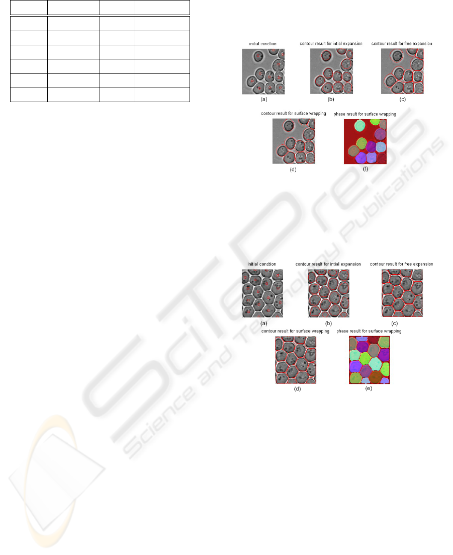
Table 4: Operation Time for Level Set Method.
Image Size ] Cell Time (sec)
1 138 ×130 11 150.43
2 140 ×120 17 235.59
3 150 ×150 19 358.29
4 176 ×139 24 455.21
5 200 ×200 31 1251.93
6 256 ×256 68 6319.55
3.6 Numerical Results
The following figures, already used in section 2.2 to
obtain the seed points, show how this method works
on real cell images. The level set method can segment
cell clusters into individual cells. The first test im-
age contains scattered cells. In Fig. 5, sub-figure (a)
shows the initial condition for level set function. Sub-
figure (b) is the result of initial expansion, in which
the fronts are located near the inner boundary of cells.
Sub-figure (c) is the result for free expansion, the
fronts are moving outside the cells but don’t penetrate
each other. Sub-figure (d) is the result for interface
wrapping, now the fronts are moving inwards until
the external boundary is detected. The last sub-figure
is the phase result of the interface wrapping, in which
all the cells are displayed with different colours. The
second test image contains clustered cells, similar as
the first test image. Fig. 6 shows the procedure of
fronts evolution. At the end, all the cells are detected
and marked with colours. This method distinguishes
the location of cells and preserves the shape of cells.
The third test image more difficult than the other two
because of the overlapping phenomenon in the image.
However, this method can still detect the location of
the cells and find out the area of the cells, the result is
shown in Fig. 7.
In all cases, one can verify that the level sets,
i.e. the individual cells, do not merge. So using this
method, the number of cells is known and the area of
each cell can be calculated. Fig. 8 is the histogram
for the test images above. Sub-figure (a) is the his-
togram for test image ”1”, there are 11 cells in the
image and they have similar size. There are two cells
smaller than others, because they are only half cells.
Sub-figure (b) is the histogram for test image ”2”, in
which contains 17 cells. From this histogram, we can
see there are four half cells. Sub-figure (c) is the
histogram for test image ”4”, 24 cells are detected,
and the ratio of the detected cells is shown in the fig-
ure. However, because of the overlapping problem,
the area is not the real area of cells, but the area of the
segmented image. Generally speaking, this method is
useful for segmenting clustered cells. By displaying
different colours for different cell regions, people can
identify cells easily.
Figure 5: Result for image 1: (a) Initial Contour; (b) Con-
tour Result for Initial Expansion (200 iterations); (c) Con-
tour Result for Free Expansion (20 iterations); (d) Contour
Result for Surface Wrapping (40 iterations); (e) Phase Re-
sult for Surface Wrapping.
Figure 6: Result for image 2: (a) Initial Contour; (b) Con-
tour Result for Initial Expansion (200 iterations); (c) Con-
tour Result for Free Expansion (10 iterations); (d) Contour
Result for Surface Wrapping (20 iterations); (e) Phase Re-
sult for Surface Wrapping.
4 CONCLUSIONS AND FUTURE
WORK
Traditional level set methods cannot segment clus-
tered cells, but only detect the boundary for groups.
We used the multiphase level set method, combining
it with the iterative voting method to segment clus-
tered cells. The iterative voting method detects the
seeds of each cell and defines it as the initial condi-
tion for the level set method. This step determines the
number of the detected cells and will influence the
performance of the level set method. Therefore, the
CLUSTERED CELL SEGMENTATION - Based on Iterative Voting and the Level Set Method
313
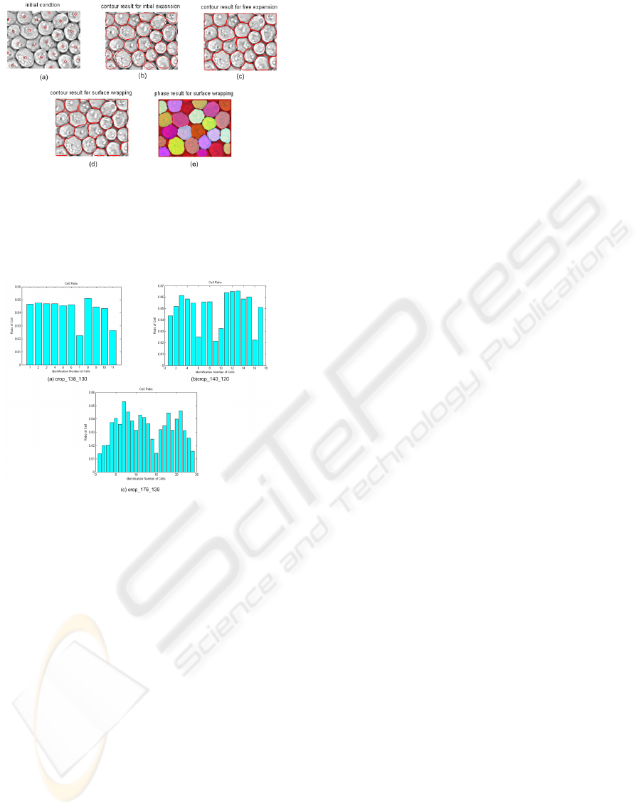
Figure 7: Result for image 4: (a) Initial Contour; (b) Con-
tour Result for Initial Expansion (200 iterations); (c) Con-
tour Result for Free Expansion (20 iterations); (d) Contour
Result for Surface Wrapping (40 iterations); (e) Phase Re-
sult for Surface Wrapping.
Figure 8: Histogram for Test Images.
parameters of this step should be chosen carefully.
The second step is to apply a level set method. For
each cell, a level set equation is set up to simulate
the seed growing procedure. In order to increase the
accuracy, a sequence of level set equations are used.
The effect of the first level set equation is to detect the
internal boundary of cells. The effect of the second
level set equation is to release the constraint and let
the fronts grow outside the cells. The effect of the last
level set equation is to move inwards the fronts and
detect the external boundary of cells. For the whole
process, reinitialisation is applied every 10 iterations,
and the reinitialisation part contains 5 steps. After
these three steps, the area of cells is detected and can
be used for further process. The drawbacks for this
approach are the time complexity and space complex-
ity. To segment n cells, n PDEs should be solved,
which requires a lot of time. When the number of
cells increases, the operation time increases sharply
and the requirement for memory also grows. There-
fore, this method is not suitable for real time applica-
tions in its current stage. As cell segmentation is usu-
ally a post-processing procedure, this is not an urgent
problem. One idea to reduce the operation time is to
use a narrow band algorithm, in which only the points
near the zero level set are updated and stored. By us-
ing this method, the program doesn’t need to update
all points in the image, but only calculates the points
near the front. The time complexity and space com-
plexity will decrease, however, presenting the loca-
tion of fronts in the program requires non-trivial work
due to the non-merging constraint.
REFERENCES
Kass, M., Witkin, A., and Terzopoulos, D. (1988). Snakes:
Active contour models. Int. J. of Comp. Vision, 1:321–
331.
Malladi, R. and Sethian, J. (1995). Level set methods for
curvature flow, image enhancement, and shape recov-
ery in medical images. In Conference on Visualization
and Mathematics, Berlin, Germany.
Mumford, D. and Shah, J. (1989). Optimal approximation
by piecewise smooth functions and associated varia-
tional problems. Comm. Pure Appl. Math, 42:577–
685.
Osher, S. and Paragios, N., editors (2003). Geometric
Level Set Methods in Imaging, Vision, and Graphics.
Springer.
Osher, S. and Sethian, J. (1988). Fronts propagating
with curvature-dependent speed: Algorithms based on
Hamilton-Jacobi formulations. Journal of Computa-
tional Physics, 79:12–49.
Sethian, J. (1999). Level set methods and fast marching
methods: Evolving interfaces in computational geom-
etry, fluid mechanics, computer vision, and materi-
als science. Cambridge University Press, Cambridge,
UK.
Solorzano, C., Malladi, R., Lelievre, S., and Lockett, S.
(2001). Segmentation of nuclei and cells using mem-
brane related protein markers. Journal of Microscopy,
201:404–415.
Sussman, M. and Fatemi, E. (1999). An efficient, inter-
face preserving level set redistancing algorithms and
its application to interfacial incompressible fluid flow.
SIAM J.Sci. Comp., 20:1165–1191.
Yang, Q., Parvin, B., and Barcellos-Hoff, M. (2004). Local-
ization of saliency through iterative voting. In ICPR
(1), pages 63–66.
Zhou, Y., Kuijper, A., Heise, B., and He, L.
(2007). Cell segmentation using the level set
method. Technical Report 2007-17, RICAM.
http://www.ricam.oeaw.ac.at/publications/reports/.
VISAPP 2008 - International Conference on Computer Vision Theory and Applications
314
