CORNER DETECTION WITH MINIMAL EFFORT ON

MULTIPLE SCALES

Ernst D. Dickmanns

Institut für Systemdynamik und Flugmechanik, LRT, UniBw Munich, D-85577, Neubiberg, Germany

Keywords: Image processing, feature extraction, corner detection.

Abstract: Based on results of fitting linearly shaded blobs to rectangular image regions a new corner detector has been

developed. A plane with least sum of errors squared is fit to the intensity distribution within a mask having

four mask elements of same rectangular shape and size. Averaged intensity values in these mask elements

allow very efficient simultaneous computation of pyramid levels and a new corner criterion at the center of

the mask on these levels. The method is intended for real-time application and has thus been designed for

minimal computing effort. It nicely fits into the ‘Unified Blob-edge-corner Method’ (UBM) developed

recently. Results are given for road scenes.

1 INTRODUCTION

(Moravec, 1979) developed the first ‘interest

operator’ for application in the field of autonomous

vehicles when computing power of microprocessors

was still very low. (Harris and Stephens, 1988)

improved the approach by looking at local intensity

gradients around the test points and by checking a

local (2 x 2) ‘structural matrix’ N defined by

products of gradient components. From the two

eigenvalues λ of this matrix, a simple criterion for

corners has been derived using

traceN =λ +λ in

combination with the determinant detN. This

approach has been the ancestor of many derivatives

(Tomasi and Kanade, 1991; Shi and Tomasi, 1994;

Birchfield, 1994; Haralick and Shapiro, 1993

) not

discussed here. Methods avoiding gradient

computation are favored lately (Smith and Brady,

1997; Drummond and Cipolla, 2002; Lowe 2004;

Rosten and Drummond, 2004). Surveys on corner

detection may be found in the bibliography (USC

IRIS, Vision Bib.com, Section 6.4.4.7) and

(http://users.fmrib.ox.ac.uk).

The approach presented here heavily relies on

gradients for its derivation, but ends up using only

four add/subtract, one division and one compare

operation for stating local nonplanarity of the

intensity function above a threshold ErrMax; the link

of this threshold to the frequently used trace of the

eigenvalues in other corner detection methods is

derived. This result is achieved by looking at a

correlation function between four local planar

approximations and one more global one (covering

the same region) as a least squares fit.

2 ROOTS OF THE NEW

APPROACH

(Hofmann, 2004) has used a set of four identically

sized rectangular mask elements (mel) for

computing edges and linearly shaded intensity

patches in an efficient way. This approach has been

expanded in (Dickmanns, 2007) by a prior non-

planarity check to separate out regions with strongly

nonplanar two-dimensional distributions of intensity.

Due to the basic regular mask structure (see bottom

of perspective projection in Figure 1) very simple

and efficiently computable results have been

obtained.

The magnitude of the errors (residues) is directly

proportional to the difference between the sums of

the intensity values on the diagonal and the counter-

diagonal, the sum of which yields the pixel intensity

on the next pyramid level:

(i, j = 1 or 2)

ij 11 22 12 21

| ε | | ( ) ( ) | / 4II II

+−+

. (1)

The average intensity I

in the mask region is

one quarter of the sum of these two diagonal sums

(= sum of all four mask elements)

315

Dickmanns E. (2008).

CORNER DETECTION WITH MINIMAL EFFORT ON MULTIPLE SCALES.

In Proceedings of the Third International Conference on Computer Vision Theory and Applications, pages 315-320

DOI: 10.5220/0001070703150320

 SciTePress

M0 11 12 21 22

()/4.I IIII= +++ (2)

Specifying a threshold level ‘ErrMax’ for this

error value for separating almost planar from

nonplanar intensity regions in the image allows

identifying potential regions for corners in the

relatively small ‘nonplanar set’. As shown in

(Dickmanns, 2007, Figures 5.23 and 5.26), for

typical road traffic scenes this reduces the areas of

interest for corner detection to only a few percent of

the entire image; with 256 intensity levels in

standard video images and with a gray value

resolution of the human eye of around 60 levels

(Darian-Smith, 1984) a threshold value around

256/60 ≈ 4 seems reasonable. Values ranging from ~

2 to 8% (4 to 20 steps in gray value) have shown

acceptable results (depending on the task).

For filtering corner candidates out of the

nonplanar set, an approach similar to (Haralick,

1993) has been used, however, with a small window

(size of the mask, see perspective projection in

Figure 1); the (2 by 2 mel) very narrow

neighborhood has its drawbacks. As a direct

consequence, results obtained are susceptible to

digitization noise when mask elements are chosen as

original pixels. Through its principle of checking the

corner conditions by diagonal sums, the method also

responds to edges in the image, the orientation of

which is close to diagonal. To separate real corners

from (noise-corrupted) digitized edges, the method

is applied again with modified parameters (see

below). TraceN has to be above a level traceN

min

guarantee the presence of a corner; traceN turns out

to be proportional to the square of the error ε

(Eq.(1)) in the present approach.

In most approaches derived from (Harris and

Stephens, 1988), the center of the region tested for

corners is a central pixel. In the approach taken in

(Dickmanns, 2007), the center of the region is the

point where all four mel meet; there is no direct

measurement value of image intensity available at

that point. Instead, the average value of mel-

intensities and their gradients are adopted for this

center point. Then, the question can been asked:

‘How do the local intensities and their gradients at

the centers of each mel correlate to the average value

at the center of the mask’. This can be investigated

with a correlation function. However, since with the

averaged planar model for the entire mask also

averaged local variations as function of y and z are

available, the correlation may be refined, asking for

deviations between the global and the local planar

models. Since the methods applied for corner

detection correspond to curvature determination via

the Hessian matrix, i.e. the second derivative of the

two-dimensional intensity function, the idea is

enhanced, whether deviations from planar relations

are not a better way to go for testing curvature. This

leads to a slightly modified correlation function as

compared to (Harris and Stephens, 1988); now the

subtracted reference is not just the average intensity

value but the averaged planar intensity model.

3 NEW APPROACH WITH A

PLANAR REFERENCE MODEL

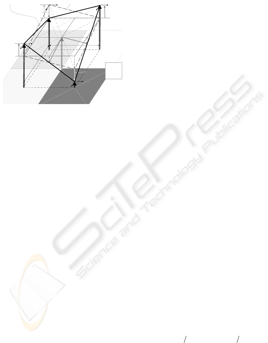
Figure 1 shows the four intensity values at the mel

centers (heavy black vertical arrows) and the

averaged intensity of the mask (gray) at the point

where all mels meet. As local intensity gradients

(Euler approximation) the differences between the

intensities of mels in row- (f

) and column direction

) are chosen (solid lines). From Figure 1, the

relations for the neighborhood of the mel centers are

obtained:

() ()

11L 11 r1 c1

12L 12 r1 c1

21L 21 r2 c1

22L 22 r2 c2

r1 12 11 r2 22 21

(,) ;

( , ) ; with

; ;

IuvI fufv

=I I m f I I m

=+⋅+⋅

−=−

(3)

−

= 2

= − 6

= 2

= − 2

= 2

= − 2

Interpolating plane with least sum of errors (

) squared

Inner reference square at

level of average intensity

Average intensity of

mask element

(2,1)

Total

mask

region

−

Local gradients at

and between mel

centers

Figure 1: Basic rectangular mask structure for fitting the

lane with least sum of errors squared (dashed gray lines)

to the four discrete intensity values I

shown as vertical

vectors. All four errors ε

are equal in magnitude and su

up to zero.

VISAPP 2008 - International Conference on Computer Vision Theory and Applications

316

(

)

(

)

c1 21 11 c2 22 12

; .

IInf IIn=− =−

The global model for the neighborhood of the

mask center can be written (Dickmanns, 2007)

MM0rc

(,)

uv I f u f v=+⋅+⋅ (4)

with

(

)

(

)

rr1r2 cc1c2

2; 2.fff fff=+ =+

The new correlation function now is

ijL M

(,) [ (,) (,)]

Euv I uv I uv=−

∑

(5)

Other than in the reference mentioned, here, absolute

intensity values are used to have the same absolute

intensities as thresholds for corner detection;

normalizing by average intensity and using a

percentage threshold favors corners in darker

regions.

The term in square brackets in Eq.(5) is written

for one mel-center with Eq.(3) and with the

abbreviation

ij ij M0

II=−

{}

11 M0 r1 r c1 c

11 r1 r2 c1 c2

{I( )( )}

Δ 0.5 [( ) ( ) ] .

Iffuffv

−+ −⋅+ −⋅

=+⋅−⋅+−⋅

(6)

Eq.(6) can be expanded to

{}

11 11 r1 r2 c1 c2

(Δ ) Δ [( ) ( ) ]

Iffuffv=+⋅−⋅+−⋅+

r1 r2

r1 r2 c1 c 2 c1 c 2

+ [ ( ) (7)

2( )( ) ( ) ]0.25.

ff u

ffffuvff v

−⋅+

⋅− −⋅⋅+− ⋅⋅

The sum S

of the mixed u·v-terms in the center

of the last row of Eq.(7) of all four intensity

components (only one shown above) can be written

r1 r2 c1 c2 r1 r2 c2 c1

r2 r1 c1 c2 r2 r1 c2 c1

()()()()

ffff ffff

Suv

ffff ffff

−−+−−+

⎡⎤

=⋅⋅⋅

⎢⎥

−−+−−

⎣⎦

Summing the terms on top of each other in this

equation yields zero so that the terms with the mixed

factor u·v vanish in the sum of Eq.(5). This leads to a

correlation function, the quadratic part of which has

no cross-products. With the help of the structural

matrix N this is written

()

22 22

r1 r2 c1 c2

r1 r2

c1 c 2

(,) .. ( ) ( )

()0

. . + .

0( )

quadr

Euv ffuffv

=+ − ⋅+ − ⋅

⎛⎞

−

⎛⎞

⎜⎟

−

⎝⎠

(8)

The trace is

r1 r2 c1 c2

()()traceN f f f f=− +− . (9)

From Figure 1 it can be seen that gradient f

(resp.

) times distance m (n) between the corresponding

mel-centers yields the intensity difference (I

– I

)

resp. (I

– I

). Therefore, the following relation

holds, relating the differences between the row

gradients to those of the column gradients

r1 c2 c1 r2

c1 c 2 r1 r 2

or ( ) / ( ).

fmf n fnf m

ff mnff

⋅+ ⋅= ⋅+ ⋅

−= ⋅−

(10)

For a square mask this means that the differences of

gradients in row and column direction are equal.

Introducing this into Eq.(9), there follows

r1 r2

()[(/)1]traceN f f m n

−⋅ +. (11)

This threshold criterion has thus been reduced to a

simple function of the difference between local row-

or column gradients, which makes sense in

connection with the interpretation of the eigenvalues

as measures of curvature of the intensity function.

For m = n (square grid) there follows a factor of 2 in

Eq.(11); circularity according to (Haralick, 1993)

then is always q = 1 here.

This has been achieved by referring curvature

to the special planar fit to the intensity function in

the mask region with least sum of errors squared.

The planarity error ε (magnitude of all residues) has

already been given by Eq.(1). Introducing this and

Eq.(10) into Eq.(11) finally yields traceN as a

function of the residue value ε of the planar fit to the

intensity function

()

16 ε .

traceN

=⋅⋅

⋅

(12)

This is the only threshold value left for adjusting the

number of corner candidates delivered by the

method; for m = n = 1 (mel = pixel), the factor to the

squared residue for obtaining traceN is 32 (Eq.(12)).

To avoid the multiplications for the comparison, of

course, the threshold value can be adjusted directly

to ε (ErrMax). The following result is thus obtained:

All quantities necessary for corner evaluation

are directly obtainable from the residue of the least

squares planar fit, which in turn is nothing but the

difference of two diagonal intensity sums in the mask

of the method UBM.

CORNER DETECTION WITH MINIMAL EFFORT ON MULTIPLE SCALES

317

4 EXPANSION TO MULTIPLE

SCALES

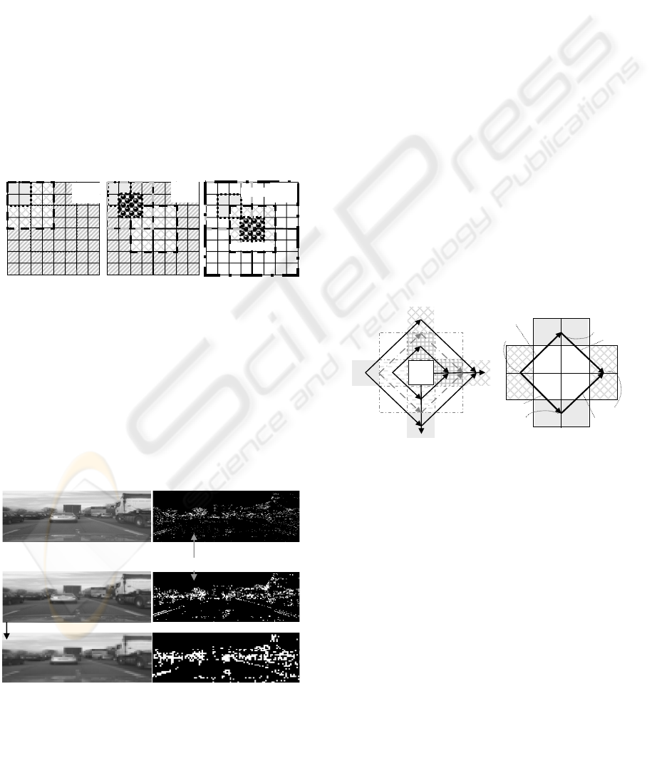
Since the base for corner detection is rather small on

the pixel grid, an extension to several pyramid levels

is desirable. This can be achieved with little

additional effort since the evaluation of the least

squares planar error according to Eq. (1) already

requires computation of the sums of the diagonal

elements. A quarter of the sum of these diagonal

sums yields the pixel intensity on the next (2 x 2)

pyramid level (1 add- and 1 shift operation).

When multiple scales are used, the center of

each pixel on the next scale is shifted relative to the

center of the previous one (see Figure 2a). The right-

hand part of the figure shows that on each pyramid

level two next-higher levels have to be computed if

pixel centers are to be placed on top of the previous

one; fortunately, this increased computational load

also saves some information from the lower level to

the next higher one if regions with sharp edges in

row- or column direction are compared.

Figure 3 shows a standard video field with its

two first pyramid levels scaled back to original size

(left). The second pyramid level already looks rather

blurred. The three images with the nonplanar regions

found by the simple method (difference of diagonal

sums larger than a threshold value) are shown on the

right-hand side. They allow the conclusion that

pyramid level one (center) may be the best scale for

detecting corners and for starting efficient

recognition of objects in real-time. On level two,

horizontal and vertical edges may be severely

blurred, depending on the position of these edges

relative to the boundaries of the pixels. Aliasing

occurs at oblique edges, leading to ‘artificial

corners’ on a local scale.

Another peculiarity to be seen from figure 3 is

the fact that edges close to diagonal satisfy the

simple ‘diagonal test’; in order to eliminate those

cases, a second test of the simple type will be

applied, however, with the sensitive direction rotated

by 45°. This second check needs only be applied to

corner candidates from the first test (a few %).

5 A SECOND TEST WITH AXES

ROTATED BY 45°

This means that now the primary gradients of

intensities are chosen as diagonals in the pixel grid

(see Figure 4); the diagonals are now horizontal and

vertical. A measurement base of rectangular shape is

used again to take advantage of the theoretical

results in plane fitting. However, the gradients are

now considered in diagonal direction.

With the planar model fit in rotated coordinates

this leads to ‘diagonal checks’ which now use one or

several pixels in the same columns or rows only.

Several arrangements are shown. On the left, single

pixels on the lowest level may be used (dark, solid

arrows) or the average of two pixels in row- or

column direction (dash-dotted gray arrows). For

these arrangements, the origin does not coincide

with the origin on the first pyramid level; the

advantage is that test values are further off the

original image diagonals, for which cases the simple

diagonal test is not able to discriminate between

edges and corners.

level 1

l e v e l 2

l e v e l 3

level 2

shift

level 1

shift

(a)

(b)

(c)

Figure 3: Computation of two images (one shifted) on nex

higher pyramid level is required, if centers of masks are to

be positioned exactly on top of each other.

Figure 2: Original video field (top left) and two 2 x 2

yramid images scaled to same size (left); right: candidate

regions for corners found by nonplanarity tests in image

intensity.

100 times residue values in perc ent (10 000 x |residue|)

second pyramid level

third pyramid level

Original video field, 768 x 287 pixels; nonplanar regions

pyramid level, 383 x 143 pixels (scaled up 2 x 2)

pyramid level, 191 x 71 pixels (scaled up 4 x 4)

dia1

cd2

dia2

cd1

refe-

rence

pixel

(i,j)

(i-1,j)

(i+1,j)

(i+2,j)

(i+1,

j+1)

(i+1,

j+2)

(i+2,

j+1)

(i+1,

j-1)

(i,j-1)

(i,

j+1)

(i,j+2)

(i-1,

j+1)

CD1

CD2

Figure 4: Rotated base (by 45°) for a second corner chec

using the model-

ased criterion from fitting a local plane

to the intensity function.

VISAPP 2008 - International Conference on Computer Vision Theory and Applications

318

The case shown on the right in Figure 4 has a

pixel on pyramid level 1 as center; the average of the

two adjacent pixels on level 0 may be taken for the

second diagonal test; however, with less effort better

results are obtained by using pixels on the next

higher pyramid level.

6 COMPARISON OF EFFORT

NEEDED AND EXPERIMENTAL

RESULTS

Beside the quality of results delivered (consistency,

completeness, localization accuracy), the effort to

obtain them is a criterion for general acceptance of a

method. The new method has been investigated

extensively with special test images and with single

real-world images from video (-fields and full

images). Qualitative results look promising so that a

real-time implementation for video-rate is underway.

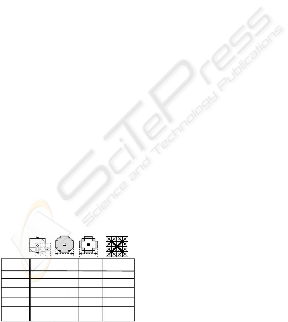
With respect to computing effort needed, Table

1 shows a comparison with other proven methods;

the corner evaluation is done for every second pixel

in total) in every second row (n

in total),

yielding m

·n

·0.25 locations. This is considered a

fair comparison to the pyramid concept in the new

method. The pyramid stages are a byproduct needing

just storage and only little additional computation

(see Eq.(2) with a single pixel as mask element).

With the size reduction by one quarter for each

stage, three stages need (1 + 0.25 + 0.0625) = 1.3125

times the operations per pixel. Assuming 15%

additional effort for removing corner candidates

stemming from nearly diagonal edges from the first

test (~ 5% of image locations and 3 times the basic

effort) requires another factor of 1.15 for the total

operations needed (~ 1.51 times the operations per

pixel, see square brackets in last column).

Table 1: Comparison of mathematical operations needed

with several corner extraction methods.

Since reusing intermediate results has been

taken into account computing the effort needed,

applying the known methods to every pixel location

requires only about doubling the numbers given. For

achieving the same localization accuracy, the new

method would have to start from twice the image

resolution, and the numbers in the last column have

to be multiplied by four. This would cut the ratio

between former and the last column in half, leaving

still some advantage to be expected for the new

method. However, since real-time visual perception

runs at 25 (33⅓) Hz with smoothing by recursive

estimation, this increased effort may not be

necessary.

Of course, these numbers can only yield a

rough estimate of computing times required by full

algorithms, since hardware capabilities and

programming proficiency also play an important role

for the results finally achieved. Future has to show

actual results.

Figure 5 shows results with two diagonal tests

but without consistent pixel centering on the

different pyramid levels. From the figure and many

other examples investigated it has been concluded

that the effort for precise superposition of mask

centers may be desirable for smooth tracking in real

time; an approach with two images on each higher

pyramid level, one shifted by (1, 1) relative to the

other (see Fig. 2), is under study and looks

promising.

Note that the approach requires no computation

of gradients at all. Just the sums of two pixels on the

diagonal have to be computed in the framework of

the fit of an intensity plane with least sum of errors

squared. The difference not only yields the residues

ε of the planar fit, but its square is also directly

proportional to the trace of the structural matrix, i.e.

the sum of the eigenvalues (Eq.(12)).

The use of two rotated planar fits allows

lowering the threshold traceN for achieving

detection of fainter real corners. If the threshold is

set too high, candidates resulting from real corners

but with low differences in intensity are lost. The

second rotated planar fit eliminates, or at least

strongly reduces, the number of candidates

stemming from noise-corrupted edges.

For real-time applications it is not so important

to detect all corners (also unreliable ones) but to

obtain sufficiently many consistent candidates for

tracking at high image rates. Edges are picked up by

separate operators anyway. Figure 5 shows that

some corner candidates are obtained on single

pyramid levels only, while others are detected on

two or even three levels; of course, these latter ones

are those best suited for tracking.

·m

·0.25

[·1.51]

·m

·0.25

·m

·0.25

·m

·0.25

number of

locations

1 [1.5]1519 361compare

1 [1.5]00 0 13mult./div.

5 [7.5]2228 5327add/subtr.

Dickmanns

2008

~ 4

FAST

2004

3.5

SUSAN

1997

2.5 3.5

Harris,

1988

~ 2.5

method,

year

radius r

16 pixel

37 pixel

2r = 2 · 3.5

−

refe-

rence

pixel

CORNER DETECTION WITH MINIMAL EFFORT ON MULTIPLE SCALES

319

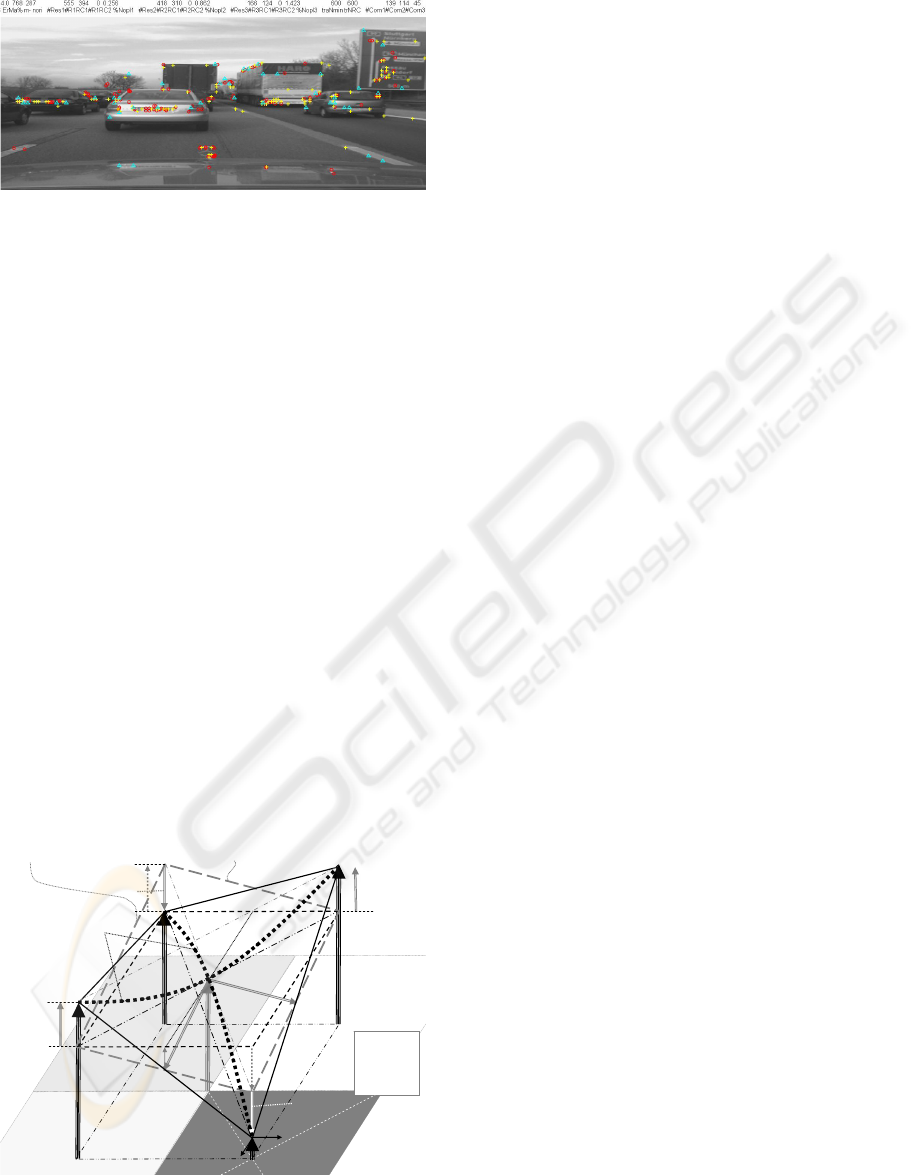
7 CONCLUSIONS

The results achieved seem to support M. Planck’s

claimed aphorism: “There is nothing more practical

than a good theory”. A least squares plane fit to the

averaged intensity surface in the area of four

identically sized elements of a rectangular mask

yields four residues of equal magnitude and opposite

signs on the diagonals. By looking at the correlation

between the averaged planar intensity function and

the local ones at the four ‘measurement points’ (I

theoretical results allow easy judgment of curvature

effects based on the eigenvalues of the structural

matrix with minimal computational efforts. Figure 6

visualizes the results obtained for saddle-point-like

corners including the curvature effects

(qualitatively), represented by the eigenvalues of the

structural matrix. (Sharp intensity spikes, of course,

tend to be lost by averaging; they are picked only

with sufficiently high spatial resolution in the

original image.)

Optimal scales (or combinations of scales) still

have to be determined from image sequences with

the real-time computing power actually available;

the results given look promising. Through the simple

nonplanarity test upfront, further corner tests may be

more involved since they have to be applied to a

small fraction of the image data only that passed the

first test. In standard road scenes, a reduction of one

to two orders of magnitude is usual.

REFERENCES

Birchfield, S., 1994. KLT: An Implementation of the

Kanade-Lucas-Tomasi Feature Tracker.

Darian-Smith, I., (ed) 1984. Handbook of Physiology,

American Physiological Society: Sensory Processes,

Vol. III, Parts 1 and 2.

Dickmanns ED., 2007. Dynamic Vision for Perception and

Control of Motion. Springer-Verlag, London.

Drummond, T., Cipolla, R., 2002. Real-time visual

tracking of complex structures. IEEE Transactions on

Pattern Analysis and Machine Intelligence, 24(7):932-

946.

Harris, C., Stephens, M., 1988. A combined corner and

edge detector. In: Alvey Vision Conference, pp 147-

151.

Haralick, R.M., Shapirom L.G., 1993. Computer and

Robot Vision. Addison-Wesley.

Hofmann, U., 2004. Zur visuellen Umfeldwahrnehmung

autonomer Fahrzeuge. Diss., UniBw Munich, LRT

http://users.fmrib.ox.ac.uk

users.fmrib.ox.ac.uk/~steve/susan/susan/node11.html.

Lowe, D., 2004. Distinctive image features from scale-

invariant keypoints. International Journal of

Computer Vision, 60(2):91-l10.

Moravec, H., 1979. Visual Mapping by a Robot Rover.

Proc. IJCAI 1079: 593-600.

Rosten, E., Drummond, T., 2004. Fusing Points and Lines

for High Performance Tracking. ICCV, pp. 1508-1511.

Shi, J., Tomasi, C., 1994. Good Features to Track. Proc.

IEEE-Conf. CVPR, pp. 593-600

Smith, S., Brady, J., 1997. SUSAN - a new approach to

low level image processing. International Journal of

Computer Vision, 23(l):45-78.

Tomasi, C., Kanade, T., 1991. Detection and Tracking of

Point Features. CMU, Tech. Rep. CMU-CS-91-152,

Pittsburgh, PA.

USC IRIS, Vision Bib.com. Annotated Computer Vision

Bibliography. Section 6.4.4.7: “Corner Feature

Detection Techniques and Use”.

Figure 6: Corner candidates from two rotated ‘diagonal

tests’ on three pyramid levels (centers not adjusted): ‘o’ =

level 0, ‘+’ = level 1, triangles = level 2. The number o

corner candidates is down to about 1/3 by the 2

test.

Figure 5: Visualization of the curvature components of the

intensity function relative to the interpolating plane

determined by the new corner detector (dotted curves).

−

= − 2

= 2

= − 2

Interpolating plane with least sum of errors (

) squared

Total

mask

region

−

Curvature

components

of intensity

surface

VISAPP 2008 - International Conference on Computer Vision Theory and Applications

320