
A NEW FACE RECOGNITION SYSTEM
Using HMMs Along with SVD Coefficients
Pooya Davari and Hossein Miar Naimi
Department of Electrical and Computer Engineering, Mazandaran University, Shariati Av, Babol, Iran
Keywords: Face Recognition, Hidden Markov Model, Singular Value Decomposition.
Abstract: In this paper, a new Hidden Markov Model (HMM)-based face recognition system is proposed. As a novel
point despite of 5-state HMM used in pervious researches, we used 7-state HMM to cover more details. As
another novel point, we used a small number of quantized Singular Value Decomposition (SVD)
coefficients as features describing blocks of face images. This makes the system very fast. In order to
additional reduction in computational complexity and memory consumption the images are resized
to
6464×
jpeg format. The system has been examined on the Olivetti Research Laboratory (ORL) face
database. The experiments showed a recognition rate of 99%, using half of the images for training. Our
system has been evaluated on YALE database too. Using five and six training images, we obtained 97.78%
and 100% recognition rates respectively, a record in the literature. The proposed method is compared with
the best researches in the literature. The results show that the proposed method is the fastest one, having
approximately 100% recognition rate.
1 INTRODUCTION
Face recognition has been undoubtedly one of the
major topics in the image processing and pattern
recognition in the last decade due to the new
interests in, security, smart environments, video
indexing and access control. Existing and future
applications of face recognition are many. A human
face is a complex object with features varying over
time. So a robust face recognition system must
operate under a variety of conditions.
There have been a several face recognition
methods, common face recognition methods are
Geometrical Feature Matching (Kanade, 1973),
Eigenfaces method (Turk and Pentland, 1991),
Bunch Graph Matching (Wiskott et al., 1997),
Neural Networks (Lin et al., 1997), Markov Random
Fields (Huang et al., 2004) and Hidden Markov
Models (Bicego et al., 2003;Kohir and Desai, 1998).
This paper presents a new approach using one
dimensional Discrete Hidden Markov Model
(HMM) as classifier and Singular Values
Decomposition (SVD) coefficients as features for
face recognition. We used a 7-state HMM to model
face configuration. Here despite of previous papers,
we added two new states to HMM to take into
account the hair and eyebrows regions. The
proposed approach has been examined on Olivetti
Research Laboratory (ORL) database. To speed up
the algorithm and reduce the computational
complexity and memory consumption along with
using small number of SVD coefficients we resized
the
92112
×
pgm formatted images of this database
to
6464
×
jpeg images. Image resizing results in
information losing and therefore seems to reduce the
recognition rate. But we have gained 99%
classification accuracy while speeding up the system
considerably. We also have examined the proposed
system on YALE face database. We resized YALE
database from
195231
×
pgm format into
6464
×
jpeg face images as well. Using five and six training
images, we obtained 97.78% and 100% recognition
rates respectively, a record in the literature.
The rest of the paper is organized as follows. In
Section 2, Hidden Markov Models and SVD are
briefly discussed. Section 3.1 describes an order-
statistic filter and its role in the proposed system.
Observation vectors calculations along with feature
extraction process are discussed in Sections 3.2 and
3.3. Section 3.4 describes feature selection method.
In Section 3.5 we introduce features quantization
and labeling process. Sections 3.6 and 3.7 represent
training and recognition procedures and discuss on
results gained on face databases. Thus Section 3
completely describes the proposed system. Finally in
Section 4 conclusions are drawn.
200
Davari P. and Miar Naimi H. (2008).
A NEW FACE RECOGNITION SYSTEM - Using HMMs Along with SVD Coefficients.
In Proceedings of the Third International Conference on Computer Vision Theory and Applications, pages 200-205
DOI: 10.5220/0001072002000205
Copyright
c
SciTePress
2 BACKGROUND
2.1 Hidden Markov Models
A HMM is associated with non-observable (hidden)
states and an observable sequence generated by the
hidden states individually. The elements of a HMM
are as below:
•
SN =
is the number of states in the model,
where
},...,
2
,
1
{
N
sssS =
is the set of all possible
states. The state of the model at time t is given
by
S
t
q ∈
.
•
VM =
is the number of the different observation
symbols, where
},...,
2
,
1
{
M
vvvV =
is the set of all
possible observation symbols
i
v
(also called the
code book of the model). The observation
symbol at time t is given by
Vo
t
∈
.
Each observation vector is a vector of observation
symbols of length T. T is defined by user based on
the in hand problem.
•
}{
ij
aA =
is the state transition probability
matrix, where:
Nji
i
s
t
q
j
s
t
qP
ij
a ≤≤==
+
=
⎥
⎦
⎤
⎢
⎣
⎡
,1,|
1
10,
≤
≤
ij
a
(1)
Ni
N
j
ij
a ≤≤
∑
=
= 1,
1
1
(2)
•
}{ )(kb
j
B = is the observation symbol
probability matrix, where:
⎥
⎦
⎤
⎢
⎣
⎡
===
j
s
t
q
k
v
t
oPk
j
b |)(
MkNj ≤
≤
≤≤ 1,1,
(3)
•
},...,
2
,
1
{
N
π
π
π
π
=
is the initial state
distribution, where:
NiP
i
i
sq ≤≤= = 1,][
1
π
(4)
Using shorthand notation HMM is defined as
following triple:
),,(
π
λ
BA=
(5)
HMMs generally work on sequences of symbols
called observation vectors, while an image usually is
represented by a simple 2D matrix.
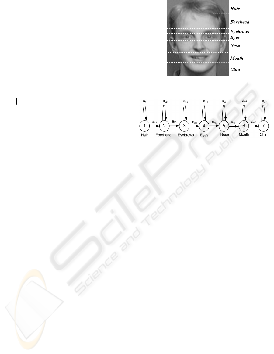
In this paper we divided image faces into 7
regions which each is assigned to a state in a left to
right one dimensional HMM. Figure 1 shows the
mentioned seven face regions.
Figure 1: Seven regions of face coming from top to down
in natural order.
Figure 2: A one dimensional HMM model with seven
states for a face image with seven regions.
Figure 2 shows equivalent one-dimensional HMM
model for a partitioned image into seven distinct
regions like Figure 1. The main advantage of the
model above is its simple structure and small
number of parameters to adjust. For a deep study on
HMMs the reader may refer to (Rabiner, 1989).
2.2 Singular Value Decomposition
The Singular Value Decomposition (SVD) has been
an important tool in signal processing and statistical
data analysis. As singular vectors of a matrix are the
span bases of the matrix, and orthonormal, they can
exhibit some features of the patterns embedded in
the signal. SVD provides a new way for extracting
algebraic features from an image.
A singular value decomposition of a
nm
∗
matrix X is any function of the form:
T
VUX Σ= ,
(6)
where
)( mmU
×
and )( nnV
×
are orthogonal matrix,
and
Σ
is and nm
×
matrix of singular values with
components
ji
ij
≠
=
,0
σ
and
0>
ii
σ
. Furthermore, it
can be shown that there exist non-unique matrices U
and V such that
0...
2211
≥≥
σ
σ
. The columns of the
orthogonal matrices U and V are called the left and
right singular vectors respectively; an important
property of U and V is that they are mutually
orthogonal. Singular values represent algebraic
properties of an image (Klema and Laub, 1980).
A NEW FACE RECOGNITION SYSTEM - Using HMMs Along with SVD Coefficients
201
3 THE PROPOSED SYSTEM
3.1 Filtering
Most of the face recognition systems commonly use
preprocessing to improve their performance. In the
proposed system as the first step, we use a specific
filter which directly affects the speed and
recognition rate of the algorithm. Order-statistic
filters are nonlinear spatial filters. A two
dimensional order statistic filter, which replaces the
centered element of a
33× window with the
minimum element in the window, was used in the
proposed system. It can simply be represented by the
following equation.
)},({
),(
min),(
ˆ
tsg
xy
Sts
yxf
∈
=
In this equation,
),( tsg is the grey level of
pixel
),( ts and
xy
S
is the mentioned window. Most
of the face databases were captured with camera
flash. Using the flash frequently caused highlights in
the subjects eyes which affected the classification
accuracy (Haralick and Shapiro, 1992). According to
sentences above, this filter is expected compensate
the flash effect (see Figure 3). It also reduces salt
noise as a result of the min operation.
3.2 The Observation Vectors
Since HMMs require a one-dimensional observation
sequence and face images are innately two-
dimensional, the images should be interpreted as a
one dimensional sequence. The observation
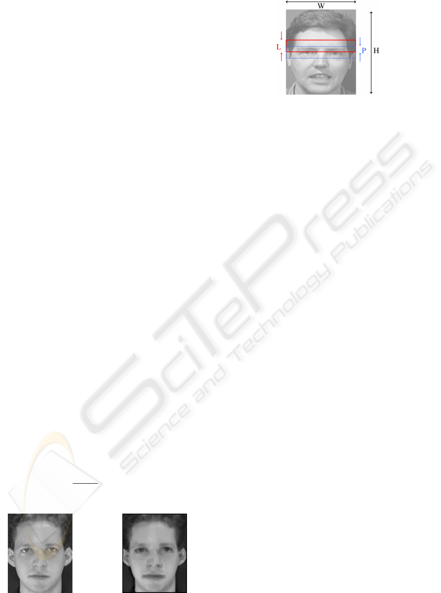
sequence is generated by dividing each face image
of width W and height H into overlapping blocks of
height L and width W. The technique is shown in
Figure 4. These successive blocks are the mentioned
interpretation. The number of blocks extracted from
each face image is given by:
1+
−
−
=
P
L
LH
T
,
(8)
where P is overlap size of two consecutive blocks.
(a) (b)
Figure 3: An example of operation of the order static filter.
Image before filtering in (a) and after filtering (b).
Figure 4: The sequence of overlapping blocks.
A high percent of overlap between consecutive
blocks significantly increases the performance of the
system consequently increases the computational
complexity. Our experiments showed that as long as
P is large (
1
−
≤
L
P
) and 10/HL ≈ , the recognition
rate is not very sensitive to the variations of L.
3.3 Feature Extraction
In order to reduce the computational complexity and
memory consumption, we resize both face databases
into
6464
×
which results in data losing of images,
so to achieve high recognition rate we have to use
robust feature extraction method.
A successful face recognition system depends
heavily on the feature extraction method. One major
improvement of our system is the use of SVD
coefficients as features instead of gray values of the
pixels in the sampling windows. We use a sampling
window of 5 pixels height and 64 pixels width, and
an overlap of 80% in vertical direction. Using pixels
value as features describing blocks, increases the
processing time and leads to high computational
complexity. In this paper, we compute SVD
coefficients of each block and use them as our
features.
3.4 Feature Selection
The problem of feature selection is defined as
follows: given a set of d features, select a subset of
size m that leads to the smallest classification error
and smallest computational cost. We select our
features from singular values which are the diagonal
elements of
∑
. It has been shown that the energy
and information of a signal is mainly conveyed by a
few big singular values and their related vectors.
Figure 5 shows the singular values of a
6464 × face
image. Obviously the first two singular values are
very bigger than the other ones and consequently,
based on the SVD theory, have more significance.
Figure 6 shows a face image along with its five
approximations, using different combinations of the
first three singular values and their related vectors.
(
7
)
VISAPP 2008 - International Conference on Computer Vision Theory and Applications
202
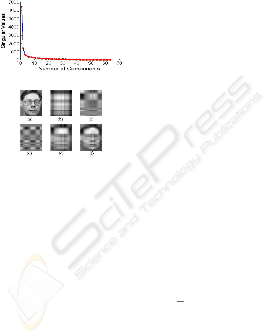
Figure 5: SVD coefficients of a
6464 ×
face image.
Figure 6: a)Original image, b)
T
vu
111
σ
, c)
T
vu
222
σ
, e) b+c
and f) b+c+d are approximations of the original image.
The last approximation (Figure 6f) contains all
three singular values together and simply shows the
large amount of the face information. To select some
of these coefficients as feature, a large number of
combinations of these were evaluated in the system.
As expected, the two biggest singular values along
with u
11
have the best classification rate.
Based on the above discussion we use two first
coefficients of matrix
∑
and first coefficient of
matrix U as three features (
11
,
22
,
11
u
σσ
)
associating each block. Thus each block of size 320
pixels, is represented by 3 values. This decreases
computational complexity and sensitivity to image
noise, changes in illumination, shift or rotation.
3.5 Quantization
The SVD coefficients have innately continuous
values. These coefficients build the observation
vectors. If they are considered in the same
continuous type, we will encounter an infinite
number of possible observation vectors that can’t be
modeled by discrete HMM. So we quantize the
features described above. To show the details of the
quantization process, used in the proposed system,
consider a vector
),...,
2
,
1
(
n
xxxX =
with
continuous components. Suppose
i
x is to be
quantized into
i
D distinct levels. So the difference
between two successive quantized values will be as
equation x.
i
D
i
x
i
x
i
minmax
−
=Δ
(9)
max
i
x and
min
i
x are the maximum and minimum
values that
i
x gets in all possible observation
vectors respectively.
][
min
i
ii
quantized
i
xx
x
Δ
−
=
(10)
At last each quantized vector is associated with a
label that here is an integer number. Considering all
blocks of an image, the image is mapped to a
sequence of integer numbers that is considered as an
observation vector. In this paper we quantized the
first feature
)(
11
σ
into 10, the second feature )(
22
σ
7
and the third one
)(
11
u into 18 levels, leaving 1260
possible distinct vectors for each block.
3.6 The Training Process
After representing each face image by observation
vectors, they are modeled by a 7-state HMM shown
in Figure 2. Five images of the same face are used to
train the related HMM and the remaining images are
used for testing.
A HMM is trained for each person in the
database using the Baum-Welch algorithm (Rabiner,
1989). At the first step
),,(
π
λ
BA=
is initialized.
The initial values for A and
π
are set due to the left
to right structure of the face model corresponding to
Figure 2.
The initial values for A and
π
are as follows:
1
0
1
7,7
615.0
1,
,
=
=
≤≤
=
+
=
π
a
i
ii
a
ii
a
(11)
Initial estimates of the observation probability
matrix B are obtained as following simple Matlab
statement:
),(
1
MNOnes
M
B =
(12)
Where M is the number of all possible
observation symbols obtained from quantization
procedure and N is the number of states.
After representing the images by observation
vectors, the parameters of the HMM are estimated
using the Baum-Welch algorithm which
finds
)|(max
*
λ
λ
λ
OP=
. In the computed model the
probability of the observation O associated to the
A NEW FACE RECOGNITION SYSTEM - Using HMMs Along with SVD Coefficients
203
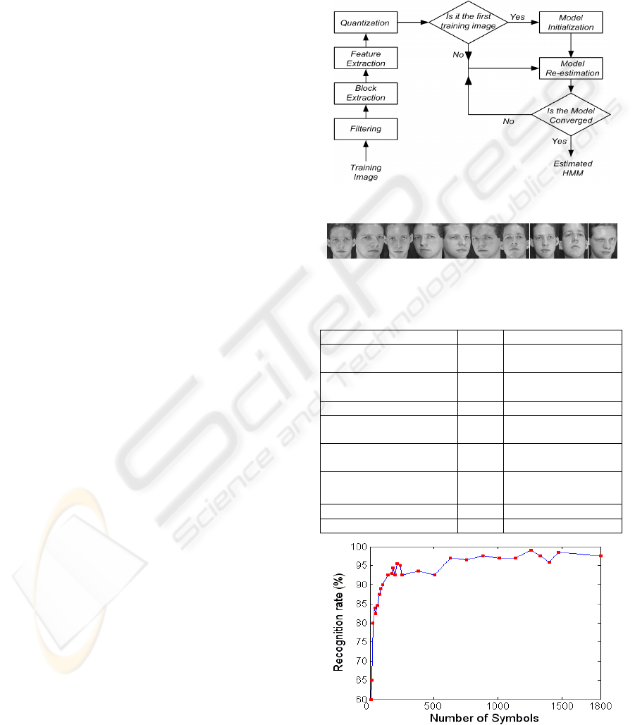
Figure 9: Showing the relation between number o
f
symbols and recognition rate. Maximum value is 99% an
d
encounter on 1260 s
y
mbols.
learning image is maximized. Figure 7 shows the
estimation process related to one learning image.
This process is iterated for all training images of a
person. The iterations stop, when variation of the
probability of the observation vector (related to
current learning image) in two consecutive iterations
is smaller than a specified threshold or the number
of iterations reaches to an upper bound. This process
is reiterated for the remaining training images. Here
the estimated parameters of each training image are
used as initial parameters of next training image.
The estimated HMM of the last training image of a
class is considered as its final HMM.
3.7 Face Recognition
After learning process, each class (face) is
associated to a HMM. For a K-class classification
problem, we find K distinct HMM models. Each test
image experiences the block extraction, feature
extraction and quantization process as well. Indeed
each test image like training images is represented
by its own observation vector. Here for an incoming
face image, we simply calculate the probability of
the observation vector (current test image) given
each HMM face model. A face image m is
recognized as face d if:
)|
)(
(max)|
)(
(
n
m
OP
n
d
m
OP
λλ
=
(13)
The proposed recognition system was tested on
the ORL face database. The database contains 10
different face images per person of 40 people with
the resolution of
92112 × pixels. As we mentioned
before in order to decrease computational
complexity (which affects on training and testing
time) and memory consumption, we resized the pgm
format images of this database from
92112
×
to
6464 × jpeg format images. Five images of each
person were used for the training task. The
recognition rate is 99%, which corresponds to two
misclassified images in whole database. Table 1
represents a comparison among different face
recognition techniques and the proposed system on
the ORL face database. It is important to notice that
all different face recognition techniques in Table 1
use
92112 × resolution of ORL face database where
we use
6464 × image size. The significance of this
result is that such a high recognition rate is achieved
using only three features per block along with image
resizing. Figure 8 shows the 10 images of one
subject from ORL face database.
We obtained 99% recognition rate by using 1260
symbols. To illustrate the relation between number
of symbols and recognition rate we varied the
number of symbols from 8 to 1800. The recognition
rate is illustrated in Figure 9. Increasing the number
of symbols to achieve greater recognition rate leads
to more time consumption for training and testing
procedure. To prevent this event we can use low
number of symbols. For example as we can see in
Figure 9 our system achieve 80%, 94.5% and 97%
accuracy respectively with 24, 182 and 630 symbols.
Figure 7: The training process of a training image.
Figure 8: A class of the ORL face database.
Table 1: Comparative results on ORL database.
Method Error Ref.
Eigenface 9.5% (Turk and Pentland,
1991)
Pseudo 2D HMM+gray
tone features
5% (Samaria and Young,
1994)
PDNN 4% (Lin et al., 1997)
Continuous n-tuple
classifier
2.7% (Lucas, 1997)
Ergodic HMM + DCT
coef.
0.5% (Kohir and Desai,
1998)
Pseudo 2D HMM +
Wavelet
0% (Bicego et al., 2003)
Markov Random Fields 13% (Huang et al., 2004)
1D HMM+SVD 1%
(Proposed method)
VISAPP 2008 - International Conference on Computer Vision Theory and Applications
204
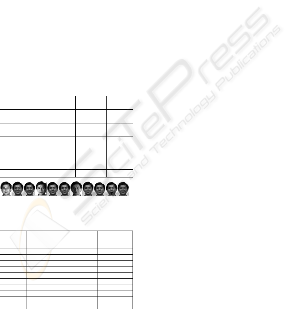
Table 2 shows a comparison of the different face
recognition techniques on the ORL face database
which reported their computational cost. As we can
see from Table 2 our system has a recognition rate
of 99% and a low computational cost. Proposed
system was implemented in Matlab 7.1 and tested on
a machine with CPU Pentium IV 2.8 GHz with 512
Mb Ram and 1 Mb system cache.
Finally we tested our system on YALE face
database. The Yale face database contains 165
images of 15 subjects. There are 11 images per
subject with different facial expressions or lightings.
Figure 10 shows the 11 images of one subject. We
resized YALE database from
195231× into 6464
×
jpeg face images. No other changes like background
cutting or cropping the images were preformed. We
obtained our system results on 1 image to 10 images
for training using 960 symbols. Table 3 shows
Comparative results on this database.
Table 2: Comparative computational costs and recognition
results of some of the other methods as reported by the
respective authors on ORL face database.
Method Recog.(%) Train. time
per image
Recog. time
per image
PDBNN
(Lin et al., 1997)
96 20min
≤
0.1 sec.
n-tuple
(Lucas, 1997)
86 0.9 sec. 0.025 sec.
Pseudo-2D HMM
(Samaria and Young,
1994)
95 n/a 240 sec.
DCT-HMM (Kohir
and Desai, 1998)
99.5 23.5 sec. 3.5 sec.
Proposed method 99 0.63 sec. 0.28 sec.
Figure 10: A class of the YALE face database.
Table 3: Experiments on YALE face database. Our
accuracy obtained on
6464 ×
resolution face images.
# of train
image(s)
MRF
(Huang et al.,
2004)
PCA
(Huang et al.,
2004)
Proposed
method
1 81.6% 60.04% 78%
2 93.11% 75.2% 82.22%
3 95.17% 79.03% 90.83%
4 95.9% 79.75% 94.29%
5 96.11% 81.13% 97.78%
6 96.67% 81.15%
100%
7 98.67% 81.9% 100%
8 97.33% 81.24% 100%
9 97.33% 81.73% 100%
10 99.33% 81.73% 100%
4 CONCLUSIONS
A fast and efficient system was presented. Proposed
system used SVD for feature extraction and 1-D
HMM as classifier. The evaluations and
comparisons were performed on the two well known
face image databases; ORL and YALE. In both
databases, approximately having a recognition rate
of 100%, the system was very fast. This was
achieved by resizing the images to smaller size and
using a small number of features.
Future work will be directed towards evaluating
the proposed system on larger face databases.
REFERENCES
Rabiner, L. R., 1989. ‘A tutorial on Hidden Markov
Models and Selected Applications in Speech
Recognition’, IEEE Proceedings, Vol. 77, No. 2, pp.
257-285.
Bicego, M., Castellani, U., and Murino, V., 2003. Using
Hidden Markov Models and Wavelets for face
recognition. In Proceedings IEEE International
Conference on Image Analysis and
Processing(ICIAP), 0-7698-1948-2.
Samaria, F.S. and Young, S., 1994. ‘HMM-based
Architecture for Face Identification’, Image and
Vision Computing, Vol. 12, No. 8,pp. 537-543.
Haralick, R.M. and Shapiro, L.G., 1992. Computer and
Robot Vision, Volume I. Addison-Wesley.
Kanade, T., 1973. “Picture Processing by Computer
Complex and Recognition of Human Faces,” technical
report, Dept. Information Science, Kyoto Univ.
Wiskott. L., Fellous, J.-M., Krüger, N., and vondder
malsburg, C., 1997. Face Recognition by Elastic
Bunch Graph Matching. IEEE Transaction on Pattern
Analysis and Machine Intelligence, 19(7):775-779.
Klema, V. C., and Laub, A. J., 1980. The Singular Value
Decomposition: Its Computation and Some
Applications. IEEE Transactions on Automatic
Control, 25(2):0018–9286.
Huang, R., Pavlovic, V., and Metaxas, D. N., 2004. A
Hybrid Face Recognition Method using Markov
Random Fields. IEEE, 0-7695-2128-2.
Kohir, V. V., and Desai, U. B., 1998. Face recognition
using DCTHMM approach. In Workshop on Advances
in Facial Image Analysis and Recognition Technology
(AFIART), Freiburg, Germany.
Turk, M., and Pentland, A., 1991. “Eigenfaces for
Recognition,” J. Cognitive Neuroscience, vol. 3, pp.
71-86.
Lin, S., Kung, S., and Lin, L., 1997. Face
Recognition/Detection by Probabilistic Decision-
Based Neural Network. IEEE Trans. Neural Networks,
8(1):114–131.
Lucas, S. M., 1997. Face recognition with the continuous
n-tuple classifier. In Proceedings of British Machine
Vision Conference.
A NEW FACE RECOGNITION SYSTEM - Using HMMs Along with SVD Coefficients
205
