TOWARDS EUCLIDEAN RECONSTRUCTION FROM VIDEO

SEQUENCES

Dimitri Bulatov

Research Institute for Optronics and Pattern Recognition, Germany

Keywords:

Calibration, Dense Reconstruction, Euclidean Reconstruction.

Abstract:

This paper presents two algorithms needed to perform a dense 3D-reconstruction from video streams recorded

with uncalibrated cameras. Our algorithm for camera self-calibration makes extensive use of the constant focal

length. Furthermore, a fast dense reconstruction can be performed by fusion of tessellations obtained from

different sub-sequences (LIFT). Moreover, we will present our system for performing the reconstruction in a

projective coordinate system. Since critical motions are common in the majority of practical situations, care

has been taken to recognize and deal with them.

1 INTRODUCTION

Considerable progress was made in the recent

years in the areas of Computer Vision and 3D-

Reconstruction from video sequences recorded with

a single uncalibrated camera. There are two princi-

pal approaches for reconstruction: the ﬁrst uses meth-

ods of projective geometry; the task is to determine

projective matrices and 3D-points in some projective

frame and then to use the additional knowledge (such

as known principal point or zero skew of the cameras)

to transform the cameras and points into a Euclid-

ean frame. In the second approach, these constraints

are imposed at the beginning, in order to avoid any

spurious results. If necessary, some additional infor-

mation is roughly estimated (such as unknown focal

length), and by the end of reconstruction, all irreg-

ularities are supposed to be corrected by means of

bundle adjustment. Examples of successfully dealing

with projectivegeometry (the ﬁrst strategy) are shown

in (Nister2001) and (Pollefeys2002). On the other

hand, (Mar2006) shows excellent results of dealing

with the second strategy. Nevertheless, many of these

algorithms are developed for ”favorable videos” and

”favorable geometry”, such as slow, smooth, almost

circular motion around a non-planar object: these al-

gorithms work well after being applied to these fa-

vorable scenes, but often turn out to be not success-

ful for almost any critical motion such as forward

motion, pure translation etc. But in reality, every

practical application of ”structure from motion” al-

gorithms – consider the area of robotics, navigation

or military applications – constantly requires dealing

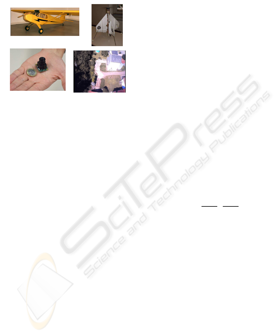
with critical motions. Our videos, recorded mostly

for military applications, are usually taken from mini-

planes or mini-drones, carrying some small cameras

(see Fig. 1), so in general, the resolution is poor, the

effects of the interlacing, lens distortion and blurring

are strong, and since the motion of these unmanned

vehicles is inﬂuenced by wind and other similar ef-

fects, the trajectory of the camera is usually not suit-

able for the reconstruction. Therefore it turned out to

be quite important to recognize and to deal with criti-

cal motions.

In many cases, we will use methods from projec-

tive geometry, see for example (HarZis2000). These

methods allow working extensively with linear equa-

tions and contribute to numerical stability and robust-

ness of the majority of the problems. In our imple-

mentation, the cameras and points in space are ob-

tained in some projective frame from interest points

detected in the images. ”Projective” means here

that the cameras and points are projectively distorted:

for example, the ratios between line segments will

not be the same as in the world coordinate frame.

Although it is not possible to recover the absolute

position, orientation and scaling of the scene just

from the video stream, our task will be to deter-

mine a 3D-rectiﬁcation homography which trans-

forms the projectively distorted model to a Euclidean

(i.e.ratio- and angle-preserving) coordinate frame.

Detecting the rectiﬁcation homography is the key-

476

Bulatov D. (2008).

TOWARDS EUCLIDEAN RECONSTRUCTION FROM VIDEO SEQUENCES.

In Proceedings of the Third International Conference on Computer Vision Theory and Applications, pages 476-483

DOI: 10.5220/0001072304760483

 SciTePress

Figure 1: a) mini-plane, b) mini-drone M3D (product of

EADS LFK) carrying small cameras c) used for recording

cityscapes as shown in d). Note the effects of interlacing,

blurring and lens distortion.

point of our method: if it works well, the object will

be clearly recognizable and all additional (rather time-

consuming) steps, such as bundle adjustment in or-

der to reﬁne the results or tessellation for better visu-

alization can optionally follow.

Notation: we denote 2D-/3D- points in the pro-

jective coordinates by column vectors: x = (x y w)

∈

, X = (X Y Z W)

∈ P

respectively. Points in

Euclidean coordinates will be denoted by

x and

X re-

spectively.

By x

, respectively

, we will refer to the point

number i in view number j. Camera matrices (to what

we shall simply refer as ”cameras”) are denoted by

P in the projective, and

P in the Euclidean frame.

We denote by K the calibration matrix, by R rota-

tion matrices and by t camera centers in the world

coordinate system. Then, the well-known relation

P = KR[I

| − t] holds. Here I

is the k × k identity

matrix.

For a matrix A, the symbols (A)

,(A)

denote the

l-th row/column of A, and (A)

{l}

,(A)

{l}

denote the

matrix after its l-th row/column has been extracted.

As usual, A

denotes the transpose of A. The opera-

tor [x]

denotes,as usually, the cross product with the

vector x.

By ℑ

, we will refer to the image contained in a

frame number r of the sequence. All other notation

will be introduced later.

Organization: in Sect. 2, we will give a brief in-

troduction of our system whose main part takes place

in the projective coordinate frame. Section 3 de-

scribes our calibration algorithm for Euclidean rec-

tiﬁcation as well as the method to perform a dense re-

contruction. Section 4 shows experimental results of

the algorithm for different kinds of video sequences.

Conclusions and outlook are given in Sect.5.

2 PROJECTIVE

RECONSTRUCTION

Given a video sequence, interest points are found in

the ﬁrst frame using Harris Corner Detector, see (Har-

ris1998) for details. Moreover, new features will be

found in periodic lags (refreshing). These features are

tracked from frame to frame by the Lucas-Kanade al-

gorithm ((KLT1981)). It is quite important to have

correspondence points over many images in order to

obtain a wide baseline. For the reconstruction, the

sequence will be automatically partitioned into sub-

sequences. The ﬁrst frame of every sub-sequence

will be called ﬁrst key-frame of this sub-sequence.

We ﬁnd the second key-frame such as the pair of

key-frames has a favorable geometry for reconstruc-

tion: we calculate two penalty terms, GRIC(F) and

GRIC(H), using formulae (2) and (3) as proposed in

(Pollefeys2003) (GRIC is the abbreviation for Geo-

metric Robust Information Criterion, introduced

by Pollefeys). Since we work with fundamental ma-

trices, the error terms ε

for the fundamental matrix

respectively ε

for the homography are:

) = max



||x



, and

) = ||

−

∗

||, x

∗

= Hx

The reconstruction begins as soon as GRIC(F) <

GRIC(H). Note that if either GRIC(F) ≥ GRIC(H)

for a rather large number of frames or the number

of points seen in the ﬁrst and in the current image

of the sub-sequence reduces dramatically, reconstruc-

tion has to be performed even though the geometry

is apparently not favorable. Once two key-frames

are determined, the fundamental matrix F between

them is calculated via RANSAC and the relative ori-

entation of two cameras is obtained as pointed out in

(HarZis2000): P

= [I

| 0

], P

= [[e

]

F | e

] where

is the epipole (projection of the ﬁrst camera center

into the second image).

The task now is to determine the points in space

(resulting from the inliers of the fundamental matrix)

and the parameters of the intermediate cameras. We

triangulate the points seen in both key-frames linearly

((HarZis2000), chapter 12) and obtain the camera ma-

trices by means of RANSAC with T

d,d

-test as de-

scribed in (Mat2004). Generating models (fundamen-

tal matrices, camera matrices, homographies) from

TOWARDS EUCLIDEAN RECONSTRUCTION FROM VIDEO SEQUENCES

477

parameter sets contaminated with outliers is an indis-

pensable part of our algorithms, so in the majority of

cases, robust methods must be applied and every pos-

sibility of speeding up the processing must be consid-

ered. Therefore, manipulating simple RANSAC by

means of T

d,d

test (with d = 1 or 2) has turned out to

be quite useful in our implementation. Also, we must

take care of critical motions since the results obtained

during this stage of reconstruction of a sub-sequence

will be used to obtain camera parameters in the fol-

lowing frames. The following observations have been

made:

• If for a large number of frames GRIG(F) >

GRIG(H), then either the scene contains some

dominant plane(s) or the baseline made up by

the cameras between two key-frames is not wide

enough. In the ﬁrst case, the linear solution for

camera resection will not work ((HarZis2000),

pp.178–180). In certain cases, one can use

homography-based reconstruction methods as

the method of camera resection by plane-by-

parallax, as proposed in (HarZis2000), chapter

18, see also (Mat2005).

• If the epipole lies inside of the image domain, the

points close to the epipole should be discarded

from triangulation, because their position in at

least one direction will be unstable. Another pos-

sibility is to take only the points which satisfy

some severe cost function such as:

∑

i=1

(

∗

−

)

< s· exp



−



, x

∗

= P

X ,

where P

are the camera matrices extracted

from the key-frames, x,X is a 2D (respectively:

corresponding 3D) point, d

is the distance from

to the epipole

and s,b are some positive con-

stants.

• The forward and backward motion usually has

both of the negative effects described above. Ac-

tually, the homography will be the suitable model

to describe the position of points in the direction

of the epipole and the epipole will be found inside

of the image. In this case, we not only discard

the points close to the epipole but also reduce the

threshold s by the factor 2.

The reconstructionof a sub-sequence continues by

extrapolation of the previous results to the frames af-

ter the second key frame. We obtain new camera ma-

trices by resection with the already known 3D-points

(via RANSAC followed by a non-linear error mini-

mization) and we obtain new 3D-points by triangu-

lation from the known cameras (usually 3–5). The

frame, where the number of either triangulation- or

resection-inliers is small, marks the end of the sub-

sequence. If the number of the unfeasible frame is

n, then the frame number n − 1 is the last frame of

the ﬁrst sub-sequence and the ﬁrst key-frame of the

next sub-sequence is n− 2. This is because we cannot

trust the camera number n of the ﬁrst sub-sequence,

and, as we will see below, we need at least a dou-

ble camera overlap. Of course, the second recon-

struction will be obtained in a different coordinate

system, therefore both reconstructions are ”fused” by

means of the common cameras P

old

n−2

old

n−1

new

and points X

new

old

seen both in old and new views.

The task is to ﬁnd a 3D-homographyH which satisﬁes

old

= P

new

H and X

old

= H

−1

new

(such a homogra-

phy exists by Theorem 9.10 in (HarZis2000)). The

method we propose works as follows:

First of all, the linear solution is calculated: if

we consider camera matrices P

old

new

H as row

vectors with 12 elements, the vector representing

the algebraic error from a single camera pair is

old

)

new

− (P

old

)

new

for k = 2, ...,12.

Clearly, each pair of projection matrices contributes

11 equations, therefore a double camera overlap is

enough to determine 16 entries of the homogeneous

quantity H. In order to reﬁne the initial value for H,

the squared geometric error

ε =

overlap

∑

j=1



new

old

−

n− j



(1)

is calculated for each 3D-points X

old

obtained in the

ﬁrst reconstruction and visible in the relevant views.

Similar error is obtained for 3D-points in the new co-

ordinate frame. Now, if the error obtained by repro-

jecting an old 3D-point with the new cameras (as in

(1) ) or vice versa is low, this point is considered to

be an inlier. In the case where there are only a few

inliers, the initial estimate of H is poor. In this sit-

uation (which, for example, can happen if the cen-

ters of both cameras coincide), we consider just a

single camera overlap P

new

old

n−2

and the correspon-

dences of reprojected points X,x, as pointed out in

(Nister2001), pp.64–65. Four such correspondences

are enough to generate a RANSAC-hypothesis from

which H can be computed. At each case, after an

initial estimate of H has been obtained, the iterative

minimization of the error given by (1) is performed

over all inliers. Given H, the new cameras and points

can be mapped into the old coordinate frame.

VISAPP 2008 - International Conference on Computer Vision Theory and Applications

478

3 AUTO-CALIBRATION AND

EUCLIDEAN

RECONSTRUCTION

3.1 Auto-Calibration

The starting point of any rectiﬁcation algorithm is a

projective reconstruction given by a set of n cam-

eras P

and points in space, X

. The task is to ﬁnd

a so called rectifying spatial homography H such as

the transformed cameras

= P

H and points

−1

represent a ratio- and angle-preserving re-

construction of the scene. If the ﬁrst camera is

given in the form P

= [I

| 0

], then, according to

(HarZis2000), pg. 460, H can be chosen as follows:

H =



K 0

−

∞

K 1



, (2)

where K is the constant but unknowncalibration ma-

trix and

∞

is the plane at inﬁnity. We store the un-

known entries of K in the column vector k = k(K) =

[ f a s u v]

, they correspond respectively to the fo-

cal length, aspect ratio, skew and two coordinates of

the principal point. There are 8 degrees of freedom

(5 for k and 3 for

∞

), so the minimization of some

geometrically meaningful cost function is to be per-

formed over the 8-tuples [k

∞

]. Before this can

be done, initial values of the parameters must be ob-

tained. At the beginning of the optimization, we set

a = s = u = v = 0. For the focal length f, the formula

obtained in (Bougnoux1998),

= −

′T

′

]

Fbb

′

′T

′

]

′

with

= diag(1 1 0),b,b

′

principal points of some

pair of cameras, F the fundamental matrix resulting

from these cameras and e

′

the epipole, can be taken

into consideration. Also, the image diagonal is an ac-

ceptable initial estimate of f. The parameters of p

∞

(the homogeneous representation of

∞

) can be es-

timated with cheirality inequalities as Nist´er pointed

out in (Nister2000s). The main theorem proved in his

paper says that if there is some plane p

which for all

i = 2,...,n satisﬁes the relation:

sgn[(p

· C(P

i−1

))(p

· C(P

))] =

sgn[(p

∞

· C(P

i−1

))(p

∞

· C(P

))] ,

(3)

then there is a continuous path from p

to p

∞

such that

no camera center is met on this path. Here we denote

by C(P) = [c

]

the camera center, normal-

ized as follows: c

= (−1)

det(P

{l}

),l ∈ {1,...,4}.

If all 3D-points have the last homogeneous coor-

dinate 1, then sgn(depth(X,P)) = sgn(w · c

) where

w = (PX)

is the third element of PX . For all points

visible by the pair of cameras P

i−1

, we calculate

= sgn[(P

)

i−1

)

]. Then, by multiplying

,i ∈ {2,...,n} by sgn



0.5+

∑



, we ensure that

the majority of X

are either in front or behind both

of the cameras (with respect to p

∞

, which in (Nis-

ter2000s) is denoted by ”untwisted pair” ). With this

normalization, all p

∞

·C(P

) must have the same sign,

so recalling (3) and setting p

· C(P

) > 0, the task is

to ﬁnd p

which satisﬁes p

· C(P

) > 0 for all i. The

problem formulated as:

• ﬁnd a maximal scalar δ subject to:

− |C





> 0 and



≤ 1,l ∈ {1,...,4}

can be solved, for example, by the Simplex Algo-

rithm. Note that the last condition allows obtaining

a unique solution for the homogeneous quantity p

This p

is an acceptable initial estimate for p

∞

be-

cause in the optimization round, we can move along a

continuous path not crossing the camera centers. We

reﬁne the initial estimate using the knowledge about

(nearly) square pixels and the principal point. Since

PH =

P = KR[I

| − t], we have (PH)

{4}

= KR. For

a matrix A, we deﬁne the operator R (A) = K/K

3,3

where K is the upper triangular matrix resulting from

the RQ-decomposition of A, in other words

K =



chol



(AA

)

−1



−1

for a non-singular matrix A. Then we know that the

matrix AK

−1

is a rotation matrix and our cost function

results in comparing R (PH)

{4}

with the ”ideal” cal-

ibration matrix diag[ f f 1] which corresponds to the

vector k

= [ f 0 0 0 0]:

∑

1≤ j≤5

1≤i≤n

k(K)

− k

(Γ

)

, K = R



H (k,

∞

)

{4}



(4)

Here H(k,

∞

) is the term for H as in (2), k

is the

new focal obtained as the result of an iteration and

are the weights representing the reliability of the

constraints. For example, we can choose Γ

= γ

where γ

is the average reprojection error of all points

observed in the camera number i and γ

say how

reliable the knowledge about camera parameters is

(we take γ

= γ

= 1,γ

= 1000 which

means that the focal length is unknown but constant).

After several iterations, the improved estimates of

skew, aspect ratio, principal point and focal length

are obtained, we update k

by k(K) in (4) and

we set γ

= 1. We optimize (4) by means of the

Levenberg-Marquardt iterative algorithm.

Remark 1. The optimization stage of auto-calibration

is fast, because all derivatives needed for the Ja-

cobian can be written analytically since the terms

TOWARDS EUCLIDEAN RECONSTRUCTION FROM VIDEO SEQUENCES

479

for the inverse of a 3 × 3 matrix and its Cholesky-

Decomposition can be performed manually. More-

over, this method usually converges after only 6–8

iterations. Other advantages of this algorithm com-

pared to other algorithms are: the fact of constant fo-

cal length is used extensively, the quality of every sin-

gle camera is taken into account and the initial value

of the plane at inﬁnity is determined in a robust way

(such as not all scene points have to lie in front of all

cameras, as for example in the case of forward mo-

tion).

3.2 Dense Reconstruction

In this subsection, we describe our method used to

generate textured maps. The points visible in the ﬁrst

key-frame ℑ of a sub-sequence are partitioned into tri-

angles (for example, by means of the Delaunay Tri-

angulation). If we assume that a triangle △

in the

image plane corresponds to a feasible (covered with

the object texture) triangle in space, we can calculate

the support plane for △

which we call ε

. If x ∈ △

then the corresponding 3D-point X can be calculated

in the projective frame either from the relation:



PX = x

X = 0 ,

(5)

or, to speed up the processing, by means of 2D-

homographies. Using operators (·)

,(·)

{l}

,(·)

{l}

deﬁned above, we have:

Result. Any of three homographies



(P)

{l}

− (P)

· (ε)

{l}

/(ε)



−1

such as ε

6= 0,l ∈ {1,2,3}, maps the triangle in image

ℑ into the corresponding triangle in space. The point

X corresponding to x is obtained as follows:

(X)

{l}

= H

x,(X)

= −(ε)

{l}

· (X)

{l}

/(ε)

To prove the formula above, we consider (5), and

we extract (X)

from its second equation. Now we

insert (X)

= −(ε)

{l}

· (X)

{l}

/(ε)

into the ﬁrst equa-

tion and obtain x = H

−1

(X)

{l}

. We only allow l ∈

{1,2, 3}, because we suppose that the Euclidean re-

construction is given on this stage, so X has the last

coordinate 1.

For better numerical conditioning, we choose l =

argmax(|(ε

)|),k ∈ {1,2, 3}. Now we can store the

numbers l

, planes ε

and the corresponding homo-

graphies H

for every triangle △

. Also, we sta-

bilize the calculations by selecting dominant planes

(via RANSAC), correcting the positions of 3D-points

and preferring the triangles lying completely in these

planes. Now, obtaining an initial hypothesis of every

pixel

x inside of the convex hull of all detected points

can be performed rather quickly, as pointed out in the

scheme below:

x → △

→ l,H

,ε

→

X (6)

Then, the unfeasible triangles can be detected by the

back-projection of the hypothesized points X into the

images close to ℑ. If the scene is not too homoge-

neous, then the intensity differences between the out-

liers must be large. Let n the number of images to

compare (n = 3–5 in our experiments), ℑ

our refer-

ence image and ℑ

,...,ℑ

images used to determine

the feasibility of △

⊆ ℑ

. Let A

be the total number

of local overlaps (how many times a point from △

was projected inside the images ℑ

,...,ℑ

). The cost

function we use to determine the feasibility of △

is:

ε( j) = (2− ξ

)log(A

)

−2

∑

x∈△

i=2,...,n

(

x,i)

, (7)

where δ

(

x,i) = ℑ

(U(

x)) − ℑ

(U(

X)) is the inten-

sity difference inside of a small window U around a

relevant pixel and ξ

is zero if △

does not lie inside

one of the dominant planes and 1 if it does. All tri-

angles, for which the cost function does not exceed a

given threshold, are declared as feasible. Contrary to

(MorKan2000) who proposes optimizing the results

of the triangulation over all possible triangulations,

we prefer use the 3D-points generated from other sub-

sequences in order to ﬁll the holes caused by unfea-

sible triangles. This seems to be a logical approach

because partitioning the video sequences into sub-

sequences (and stitching these sub-sequences as de-

scribed in Sect. 2) is a consequence of the fact that the

object is seen from differentpositions. In order to pro-

vide the texture of every of these views, a reference

image from a sub-sequence must be taken. We call

this method ”Local Incremental Fusion of Tessella-

tions”, LIFT. Suppose we are given m sub-sequences

(i.e. reference images ℑ

,...,ℑ

for which we have

triangulations, support planes and homographies. The

task is to compute the feasibilities for the triangles

of the last sub-sequence. The computation algorithm

works as follows (s

are constant thresholds):

for every pixel

x =

in ℑ

determine j such as

x ∈ △

extract ε

and H

, then calculate

X using (6)

increase area A

and set status = 0;

for i = 1, ...,m− 1

reproject

X with camera

to obtain

lies inside of a feasible triangle in ℑ

compare the support plane ε of this triangle with ε

if ||ε- ε

|| < s

(it is approximately the same point)

increase overlap

, set status = 1 and break

if status == 0

VISAPP 2008 - International Conference on Computer Vision Theory and Applications

480

(an occluded point or is not inside of all previous images)

reproject

X into the neigboring images ℑ

,...,ℑ

calculate intensity differences proceeding from

x with (7)

add the squared sum of these errors to δ

for every j

if overlap

> s

or ε

> s

(as in (7))

the triangle j is declared unfeasible

Finally, feasible triangles from all sub-sequences

will be given their texture, as shown in the images

below.

4 RESULTS

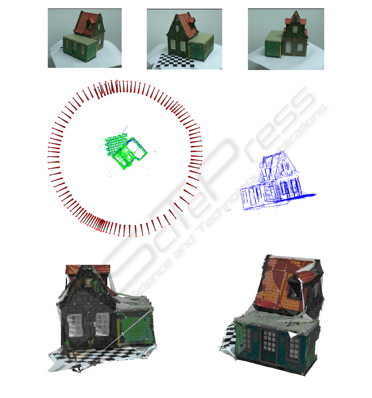
We will present results from three movies taken with

three different cameras. The ﬁrst movie (”House”,

400 frames, 105 camera positions – because every 4-

th frame was taken) was recorded with a handheld

camera around a toy-house, so its resolution as well

as the trajectory of the camera is good. The only

difﬁculties the system has to deal with are the large

number of outliers and the conﬁguration of inliers: in

many frames they are nearly coplanar which makes

the camera resection quite difﬁcult. The result of the

calibration algorithm is illustrated in two Fig. 2, with

the texturation obtained with our method of local in-

cremental fusion LIFT.

The second sequence (”Infrared”, some 150

frames) was recorded by an infrared camera and

shows a sky-scraper in Frankfurt-upon-Oder. As in

most infrared sequences, the percentage of tracking

outliers is large, due to dead pixels. Moreover, al-

most all of the 3D-points are situated either far away

from the object or in some dominant planes, which

makes the usual determination of p

∞

quite hard. Nev-

ertheless, the result of our calibration algorithm was

reﬁned by bundle adjustment, and the results of our

method are shown in Fig.3.

The sequence (”Cityscape”, 20 frames) is ob-

tained from our mini-plane and shows a typical view

of a cityscape as in Fig. 1. Also here, the results of

reconstruction are good (Fig. 4) compared with the

quality of the input video.

In all sequences, the calibration matrix was very

close to what we have estimated by using a calibra-

tion plane, therefore we can assume that the small de-

viations were caused by lens distortion effects. The

small effects of projective distortion in the sequence

”Infrared” were eliminated by means of bundle ad-

justment.

5 CONCLUSIONS AND FUTURE

WORK

Conclusions. We have presented a system which is

able to perform the Euclidean reconstruction from

video sequences recorded with a single camera. The

system can recognize some important critical motions

(such as forward and backward motion) and deal with

them, such that even in the case of not favorable

geometry, the results of reconstruction are acceptable.

Another advantage is that the system is robust: for ex-

ample, outliers caused by small moving objects in the

images will be detected by robust algorithms and ex-

cluded from consideration.

The structure of the system allows detecting and

tracking points, performing and stitching projective

reconstructions from frame to frame. In other words,

there is no need of exhaustive matching of pairs or

triples of frames (as in (Mar2006) or (Nister2000)) to

ﬁnd a pair or a triple with a favorable geometry. The

reconstruction can be stopped anytime, if necessary,

given that the reconstruction between the ﬁrst pair

of key-frames was performed. Then, the calibration

process is quite fast and as result, a sparse cloud of

3D-points and the camera trajectory will be obtained.

The computation times of the ﬁrst draft of our algo-

rithm lie between 10 and 15 frames/sec., therefore the

hope to achieve a real-time reconstruction exists. Ex-

tracting and fusing dense models obtained from sev-

eral sub-sequences as described above is also a fast

process (because the optimization is performed over

triangles rather than over points), but before this can

be done, the error minimization over all points and

all cameras must be performed to optimize the results

of the sparse reconstruction which is a rather time-

consuming process.

Future Work. Our next step towards the dense re-

construction will be the search of a global algorithm

which considers the triangulation from the reference

frames of all sub-sequencesat the same time and deals

with occlusions. The task is to reﬁne the initial result

obtained by LIFT. Thus, the local cost function given

by (7) has to be modiﬁed. Still, our biggest prob-

lem remains the quality of our videos. We deinter-

lace the images, if necessary, but the blurring effects

are in many cases very strong. Lens distortion is also

a serious problem: without distortion correction, the

assumption of linear transformations between images

does not hold, so the complete reconstruction algo-

rithm is likely to collapse. At the moment, we esti-

mate the distortion coefﬁcients before the ﬂight and

undistort the images, but future work includes auto-

matic recognition and correction of lens distortion.

TOWARDS EUCLIDEAN RECONSTRUCTION FROM VIDEO SEQUENCES

481

100

101

102

103

104

105

Figure 2: Results of reconstruction of sequence ”House”: three views from the original sequence, result of sparse reconstruc-

tion given in points and straight lines and camera trajectory. Below are two snap-shots from the textured model. Note the

small number of undetected unfeasible triangles.

VISAPP 2008 - International Conference on Computer Vision Theory and Applications

482

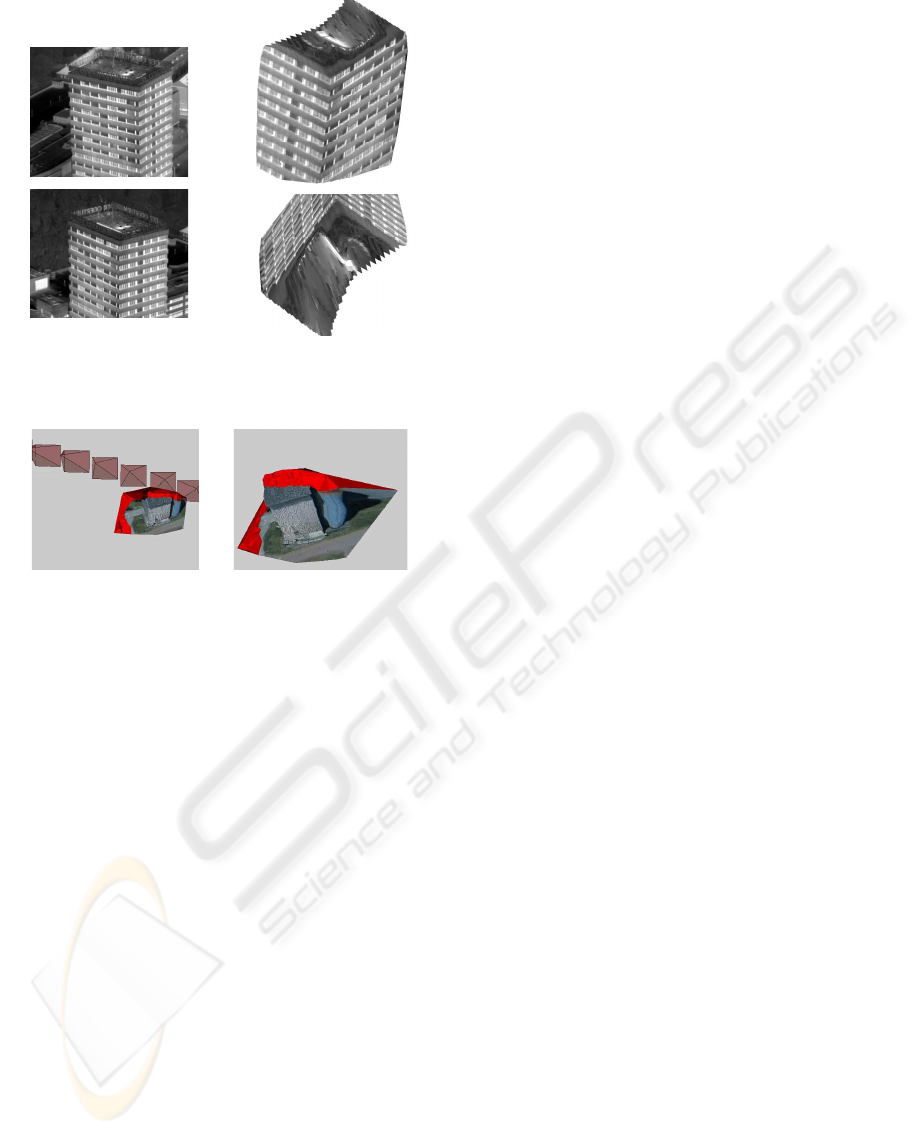
Figure 3: Results of reconstruction of sequence ”Infrared”.

Figure 4: Results of reconstruction of sequence

”Cityscape”. We show cameras trajectory and a

dense point cloud inside of the convex hull of Harris-Points

detected only in the ﬁrst view. Points outside the convex

hull are marked by red.

REFERENCES

Bougnoux S., From Projective to Euclidean space under any

practical situation, a criticism of self-calibration. In

Proceedings of the International Conference on Com-

puter Vision (ICCV), Bombay, India, pp. 790-796,

January 1998

Harris C. G., Stevens M. J., A Combined Corner and Edge

Detector. In Proceedings of 4th Alvey Vision Confer-

ence, pp.147-151, 1998

Hartley R., Zisserman A., Multiple View Geometry in Com-

puter Vision. Cambridge University Press, 2000

Lucas B., Kanade T., An Iterative Image Registration Tech-

nique with an Application to Stereo Vision. In Pro-

ceedings of 7th International Joint Conference on Ar-

tiﬁcial Intelligence (IJCAI), pp. 674-679, 1981

Martinec D., Pajdla T., 3D reconstruction by gluing pair-

wise Euclidean reconstructions, or ’how to achieve a

good reconstruction from bad images’. In Proceedings

of the 3D Data Processing, Visualization and Trans-

mission conference (3DPVT) , University of North

Carolina, Chapel Hill, USA, June 2006.

Matas J., Chum O., Randomized Ransac with T

d,d

-test. Im-

age and Vision Computing, 22(10) pp. 837–842, Sep-

tember 2004.

Matas J., Chum O., Werner T., Two-view geometry estima-

tion unaffected by a dominant plane. In Proceedings of

Conference on Computer Vision and Pattern Recogni-

tion (CVPR), Vol. 1, pp.772–780, Los Alamitos, Cal-

ifornia, USA, June 2005

Morris D. Kanade T., Image-Consistent Surface Triangu-

lation. In Proceedings of the IEEE Conference on

Computer Vision and Pattern Recognition (CVPR–

00), volume 1, pages 332–338, Los Alamitos, 2000.

IEEE

Nist´er D., Automatic dense reconstruction from uncali-

brated video sequences. PhD Thesis, Royal Insti-

tute of Technology KTH, Stockholm, Sweden, March

2001

Nist´er D., Reconstruction from uncalibrated sequences with

a hierarchy of trifocal tensors. In Proceedings of the

European Conference on Computer Vision, ECCV,

Vol. 1, pp.649–663, 2000

Nist´er D., Untwisting a projective reconstruction. Interna-

tional Journal of Computer Vision, 60(2) pp.165–183

Pollefeys M., Obtaining 3D Models with a

Hand-Held Camera/3D Modeling from Im-

ages. Tutorial notes, presented at Siggraph

2002/2001/2000, 3DIM 2001/2003, ECCV 2000,

http://www.cs.unc.edu/ marc/tutorial/

Pollefeys M., Verbiest F., Van Gool L., Surviving dominant

planes in uncalibrated structure and motion recovery.

Computer Vision – ECCV 2002, 7th European Con-

ference on Computer Vision, Lecture Notes in Com-

puter Science, Vol. 2351, pp.837–851, 2003

TOWARDS EUCLIDEAN RECONSTRUCTION FROM VIDEO SEQUENCES

483