
BINARY IMAGE SKELETON
Continuous Approach
Leonid Mestetskiy
Department of Mathematical Methods of Forecasting, Moscow State University, Moscow, Russia
Andrey Semenov
Department of Information Technologies, Tver State University, Tver, Russia
Keywords: Binary image, continuous skeleton, discrete skeleton, polygonal figure, pruning, skeletal base.
Abstract: In this paper we propose a building technique of a correct model of continuous skeleton for discrete binary
image. Our approach is based on approximation of each connected object in an image by a polygonal figure.
Figure boundary consists of closed paths of minimal perimeter which separate points of foreground and
background. Figure skeleton is constructed as a locus of centers of maximal inscribed circles. In order to
build a so-called skeletal base from figure skeleton, we cut unnecessary noise from it. It is shown, that the
constructed continuous skeleton exists and is unique for each binary image. This continuous skeleton has
the following advantages: it has a strict mathematical description, it is stable to noise, and it also has broad
capabilities of form transformations and shape comparison of objects. The proposed approach gives a
substantial advantage in the speed of skeleton construction in comparison with various discrete methods,
including those in which parallel calculations are used. This advantage is demonstrated on real images of
big size.
1 INTRODUCTION
Mathematical concept of a skeleton has been
formulated initially only for continuous objects
(Blum, 1967). A skeleton of a closed region on
Euclidean plane is defined as a set of centers of
maximal empty disks. A disk is empty if each
internal point of it is also internal point of the region.
In order to use the concept of a skeleton as a
research tool of image shape in digital images, one
needs to extend this concept to discrete space.
However, in spite of seeming simplicity, it is not
possible to extend this definition to discrete images
immediately (Smith, 1987; Ogniewicz and Kubler,
1995; Bai et al., 2007). Efficient algorithms of
continuous skeleton construction are known only for
polygonal regions (Lee, 1982; Fortune, 1987; Yap,
1987; Klein and Lingas, 1995). However, for exact
polygonal approximation of discrete form
boundaries, one needs to use many small rectilinear
segments. This leads to an increase in the number of
vertices of approximating polygons. But the more
vertices there are in polygons, the more noisy
branches of skeleton are generated. And these
branches are not important for an analysis of image
shape.
Since it is impossible to use continuous
skeleton for image analysis, «discrete skeleton», an
analogue of continuous skeleton, is constructed for
these purposes. A discrete skeleton is usually
defined as a binary image derived by a certain
transformation of the initial image. The skeleton
consists of pixel-wide lines and all of these lines are
approximately equidistance from the boundary of
the initial object. There exist several approaches of
construction of such transformation: topological
thinning, morphological erosion and allocation from
a distance map (Costa and Cesar, 2001). However,
discrete skeletons obtained by these methods have
essential disadvantages in comparison with their
continuous analogues. In methods of topological
thinning and morphological erosion the Euclidian
metric is lost. Skeletonization methods by distance
map cause loss of skeleton connection. In addition
presentation of skeletons as binary images
complicates their comparison. It is also impossible
251
Mestetskiy L. and Semenov A. (2008).
BINARY IMAGE SKELETON - Continuous Approach.
In Proceedings of the Third International Conference on Computer Vision Theory and Applications, pages 251-258
DOI: 10.5220/0001072402510258
Copyright
c
SciTePress
to transform image shape on the basis of a discrete
skeleton.
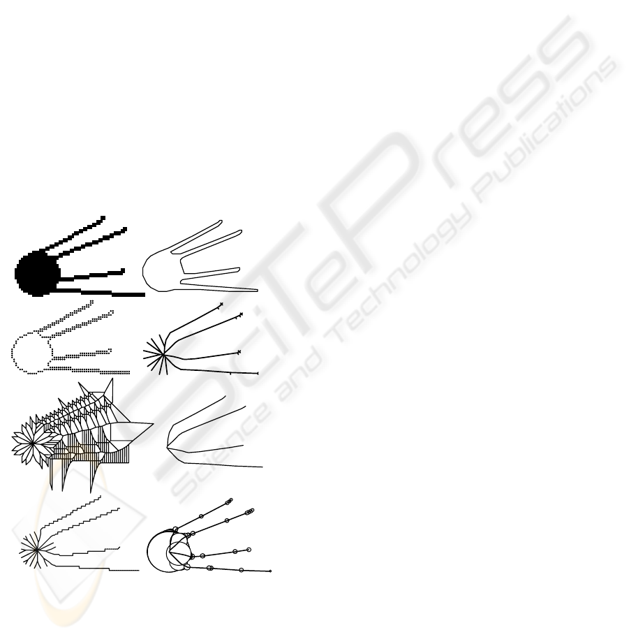
Another approach, proposed in (Ogniewicz and
Kubler, 1995), uses a subgraph of the Voronoi
diagram of object boundary points as a skeleton of a
discrete object (Fig.1(a-d)). This subgraph is
extracted from the Voronoi diagram on basis of
regularization procedure. Therefore, the resulting
continuous skeleton is a planar linear graph. Since it
is continuous and not discrete, it suits much better
for image shape transformation and comparison. The
disadvantage of the resulting skeleton is that its
branches are often zigzag. This disadvantage
becomes especially pronounced for images of low
resolution (Fig.1(d)). In addition, when this method
is applied to a complex image of high resolution,
which also has regular elements (for example, to a
drawing with rectilinear fragments), a big number of
"redundant" boundary pixels becomes involved in
processing, which leads to an unnecessary increase
in the dimension of Voronoi diagram and the total
amount of calculations.
Figure 1: (a) – the binary image, (b) – the boundary points,
(c) – the Voronoi diagram of boundary points (only finite
edges), (d) – regularization of the Voronoi diagram, (e) –
the approximating polygonal figure, (f) – the figure
skeleton, (g) – the skeleton regularization, (h) – the radius
function of skeleton.
Not only the quality of a skeleton constructed
by a specific algorithm is important. The speed with
which this algorithm works is very important in
computer vision systems. Currently speed
enhancement is usually achieved by the
development algorithms of parallel discrete
skeletonization (Manzanera et al., 1999; Deng et al.,
2000; Strzodka and Telea, 2004). However this
acceleration has its limits since there remain
sequential steps in discrete skeleton construction
algorithms and the number of these steps increases
with the growth of image size. Image size, in turn,
increases steadily as resolution of cameras and
scanners increases.
In reality, the time necessary for skeletonization
of big images even on modern computers is still too
big for many applications.
Therefore, the issue of extension of the concept
of continuous skeletons on discrete images seems far
from being resolved. The purpose of this paper is to
describe a continuous approach to skeletonization of
binary images (Fig.1(e-h)) developed by the authors
and its application to real-world problems
(Mestetskiy, 1998, 2000, 2006). The advantages of
the proposed method are also demonstrted in the
paper. The main advantages include superiority in
computer efficiency.
2 DISCRETE FIGURE AND ITS
SKELETON
We will define a skeleton of a discrete image on the
basis of the following concepts:
- а discrete figure;
- аn approximating minimal perimeter polygonal
figure;
- а continuous skeleton of a polygonal figure;
- а skeletal base of a polygonal figure.
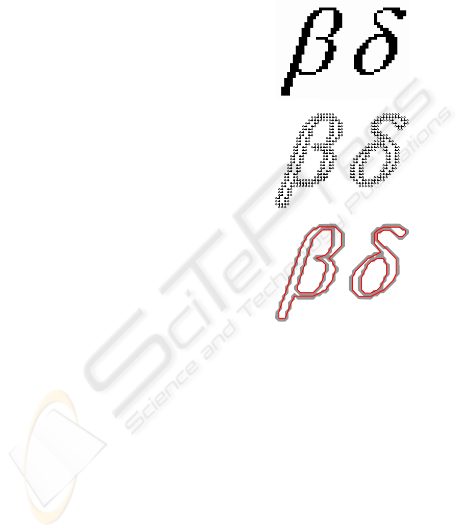
2.1 Discrete Figures in Binary Image
A binary image is a two-colored picture where one
or several objects of one color are located on a
background, which has another color. Without loss
of generality, we will consider a binary image as a
black-and-white image: object is black, and
background is white. Such image is represented in a
computer as a matrix of black and white pixels.
Let us define an adjacency structure on a set of
pixels as follows. For a black pair of pixels we will
define neighborhood as 8-adjacency, and for a white
pair and a two-colored pair – as 4-adjacency.
(a)
(b)
(c)
(d)
(e)
(f)
(g)
(h)
VISAPP 2008 - International Conference on Computer Vision Theory and Applications
252
A set of one-colored pixels is called connected
if for each pair of pixels in it there is a path from one
pixel to another, consisting of sequentially
neighboring pixels of the same color. Maximal
connected set of pixels of one color is called a
connected component. If all pixels of a component
lie on the same straight line, such a component is
called degenerated. Let us define discrete figures as
connected black-colored components. There are 5
connected components in the image in Fig.2(a), two
of them are discrete figures.
2.2 The Continuous Approximation of
Discrete Figure
Let us regard pixels as points with integer co-
ordinates on Euclidean plane.
We will call a pair of 4-adjacent two-colored
points a boundary pair, a segment connecting these
points – a boundary segment. Two components to
which points of a boundary pair belong are called
adjacent, and the boundary pair is called dividing for
these components. The set of all dividing boundary
pairs for two adjacent components we will name a
boundary corridor (Fig.2(b)). Each discrete figure
defines one or more boundary corridors.
Let us say, that a closed path lies in a boundary
corridor if it crosses all boundary segments of this
corridor. We will consider that a path crosses a
segment if it has a common point with it and lies on
different sides from this segment in some
neighborhood of the intersection point. There will
exist a minimal length path in the set of paths lying
in a boundary corridor. This path will be a closed
polyline and we will call it a separating minimal
perimeter polygon (MPP). If a discrete figure and all
its holes are not degenerated then all its MPP are
simple polygons (Fig.2(c)). For a degenerated figure
or a degenerated hole MPP degenerates in a line
segment. The set of all MPP of a discrete figure
defines a polygonal figure – «a polygon with
polygonal holes».
Thus, we have defined minimal perimeter
polygonal figures that approximate discrete figures
of binary image. It is important to note that the set of
approximating polygonal figures always exists and
is unique for a given binary image.
2.3 Polygonal Figure Skeleton
Degenerated disks of zero radiuses centered in the
convex vertices of a polygonal figure are empty as
they have no internal points and, therefore, don’t
contain boundary points of a figure. Besides, they
are the maximal empty disks since they don’t
contain other empty disks. Therefore points, which
coincide with convex vertices of a polygonal figure,
belong to a polygonal figure skeleton.
(a)
(b)
(c)
Figure 2: (a) – the binary image with 5 components and 2
discrete regions, (b) – boundary corridors, (c) – minimal
perimeter polygons.
A polygonal figure skeleton is a planar graph
with edges consisting of line segments and parabolas
(Lee, 1982). The vertices of this skeleton are
comprised from the convex vertices of a polygonal
figure (one degree vertices) and from the points,
which are centres of the inscribed circles, tangent to
figure boundary in three or more points (three and
more degree vertices). The radial function is defined
in each skeleton point as the radius of an inscribed
circle centered in this point.
It is important to underline that a polygonal
figure skeleton always exists and is unique.
2.4 Polygonal Figure Skeletal Base
The problem of “noise” branches exists for both
continuous and discrete skeletons. Small
BINARY IMAGE SKELETON - Continuous Approach
253
irregularities in figure boundary lead to occurrence
of skeleton branches, unessential for analysis of
image form. The task of skeleton regularization is to
remove these branches and leave only fundamental
part of the skeleton which at the same time
characterizes properties of the shape. This
fundamental part looks like a skeleton subgraph. We
will name it a skeletal base. Since the transformation
of a skeleton into a skeletal base is achieved by the
removal of unessential vertices and edges, this
process is called pruning.
Let C be a polygonal figure. Let us call its
boundary ∂C, its skeleton – S and its skeleton radial
function –
ρ
(s), s∈S. The skeleton will be a planar
graph
),( EPS = with the set of vertices P and
edges E. We will call a skeleton vertex with one
incident edge terminal, and with two or more edges
– internal. An edge incident to a terminal vertex is
also called terminal; an edge incident to two internal
vertices is called linking. Linking edges can enter in
one or more cycles and in this case they are called
cyclic.
Pruning is a consecutive removal of some
terminal vertices and skeleton edges incidental to
them. In the process of pruning, degree of some
vertices changes. In particular, internal vertex can
become terminal or its degree can become 2.
Pruning guarantees preservation of skeleton
connectivity and also preservation of all cycles in a
skeleton as it doesn’t touch cyclic edges.
Let us consider an assessment criterion of
“essentiality” of a terminal edge. Essential edges
remain in a skeletel base, and unessential edges are
cut.
Let
),( EPS
′′
=
′
be some adjacent subgraph
of a skeleton
),( EPS = , such that PP ⊆
′
,
EE ⊆
′
and also such that in the set EE
′
\ there
are no cyclic edges of skeleton. This means, that
graph
S
′
can be obtained from skeleton S by the
removal (“pruning”) of some vertices and edges of
skeleton, and such removal doesn’t destroy cycles
and doesn’t break connectivity of the graph. This
graph
S
′
we will call truncated subgraph of
S
. We
will consider the set of points formed by union of all
inscribed circles, centered in points of the truncated
subgraph
S
′
, whose radiuses are equal
ρ
(s), s∈ S
′
.
This set of points forms a closed region which we
will call a silhouette of subgraph
S
′
. The important
property of a truncated subgraph silhouette is its
topological equivalence to figure C. In particular, a
silhouette is a connected set.
Let a skeletal base of figure C be the minimal
truncated subgraph
S
′
of its skeleton S with
silhouette
S
V
′
satisfying a condition
ε
≤
′
),(
S
VCH , where 0>
ε
is a regularizing
parameter, and
),(
S
VCH
′
– Hausdorff distance
between figure C and silhouette
S
V
′
.
It is necessary to note, that for each value of
parameter
ε
the skeletal base always exists and is
unique.
We will call the derived skeletal base a
continuous skeleton of a discrete figure.
3 ALGORITHMS
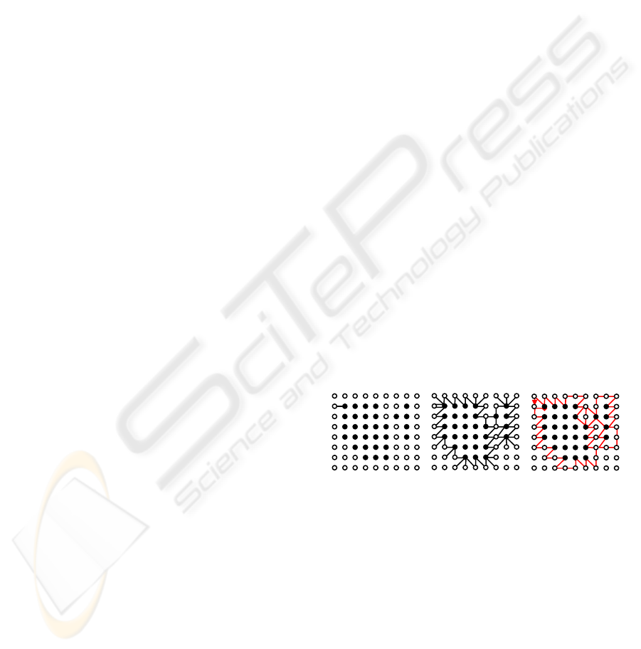
3.1 Boundary Corridor
The construction of a boundary corridor consists of
two stages: the corridor search and its tracing.
Corridor search is understood as a problem of
finding one boundary pair of points (Fig.3(a)).
Search of such pair can be executed by row scanning
of the binary image. After finding the boundary pair,
the boundary tracing algorithm will work. This
algorithm reveals all other boundary pairs of a
corridor. After corridor tracing is finished, the
algorithm starts the search of next corridor from that
location where the first boundary pair of the
previous corridor has been found. The process ends,
when the single line scanning ends.
Figure 3: Corridor tracing: (a) the initial position of tracer
pair, (b) the consecutive positions of tracer pair, (c) the
sequence of test points (tracing track).
The algorithm starts contour tracing from the
first boundary pair and finds sequentially other
boundary pairs of a corridor. A boundary pair of
points currently found by the algorithm we will call
a tracer pair. Tracing process corresponds to the
consecutive movement of the white end of the tracer
pair in a positive direction relative to the black end
(Fig.4). The derived point is called a test point. All
possible variants of test point choice at different
positions of the tracer pair are presented on Fig.4.
(a)
(b)
(c)
VISAPP 2008 - International Conference on Computer Vision Theory and Applications
254
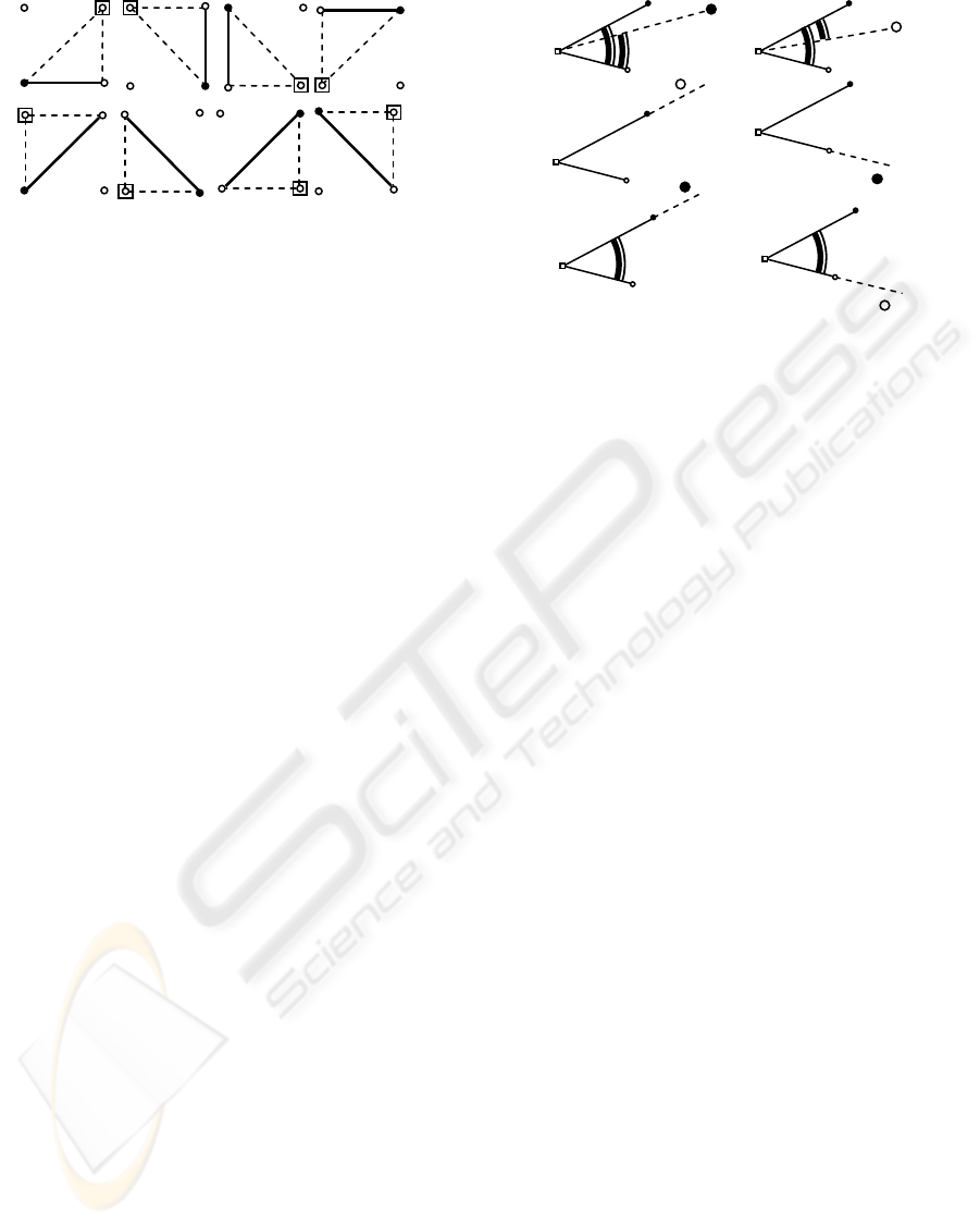
Current position of the tracer pair is shown by a
solid line, and new possible positions depending on
color of a test point – by a dotted line.
A new position of a tracer pair is determined
from the color of a test point by the following rule.
The test point replaces in the tracer pair a point of
the same color as it is.
Consecutive moving of a tracer pair allows to
single out all boundary points corresponding to one
boundary contour (Fig.3). Tracing process ends
when tracer pair will return to its initial position.
3.2 Minimal Perimeter Polygon
The sequence of test points forms an ordered list
called a tracing track (Fig.3(c)). We will attain
"walls" of a boundary corridor by sequentially
connecting all black points of this list among
themselves and all white points. The left wall
consists of black points, and the right one – of white
points. The minimal perimeter polygon lies between
the corridor walls. All vertices of MPP are points of
a tracing track. We will call such points a corner.
The task of MPP construction is to choose corner
points from a tracing track.
The first corner point is defined from the initial
position of the tracer pair (Fig.3(a)). It is obvious,
that the right point of this pair is always corner. Let
us note, that the two consecutive vertices in MPP
should be connected by line segment lying between
corridor walls completely. It means, that if another
(in particular, the first) corner point is found, it is
necessary to search for the next corner point as for a
point lying from it «in the line of sight» inside a
corridor.
Let us define a concept of a «coverage sector»
for a corner point. At the initial moment (for the
current found corner point) it equals 360 ° and isn’t
limited by anything. As the algorithm proceeds, the
points of the track after this corner point are
sequentially considered and the coverage sector is
modified by following rules (Fig.5):
1. If the test point is located inside the coverage
sector, the sector changes (Fig.5(a,b)). If the test
point is black (Fig.5(a)), it is declared as the left side
of the sector, if it is white (Fig.5(b)) – as the right
one.
2. If the white point is located outside the
coverage sector to the left of its left side (Fig.5(c)),
the left black point of the sector is declared the new
corner point. Similarly, if the black point is located
outside the sector to the right of its right side
(Fig.5(d)), the right white point is declared the new
corner point.
3. In all other cases (Fig.5(e,f)) the coverage
sector doesn’t change.
As these rules are followed, all corner points
are sequentially found. In the process, the corridor
track is regarded as a circular list of points. The
process ends when the initial corner point is chosen
as a new corner point (but not as a test point!) once
again.
3.3 The Construction of Skeletons
Fast algorithms for skeleton construction of simple
polygons with n vertices have computational
complexity O (n log n) (Lee, 1982) and O (n) (Klein
and Lingas, 1995). Known generalizations to the
case of a polygonal figure with holes (Srinivasan et
al., 1992, Lagno and Sobolev, 2001) have
computational complexity O (kn + n log n), where k
is the number of polygonal holes and n is the general
number of vertices. For some problems such
computational complexity takes too much. For
example, in the task of construction of an external
skeleton for segmentation of the text document
(c)
(d)
(a)
(b)
(
e
)
(
f
)
Figure 4: Choice of the next test point (labeled as square)
for different positions of tracer pair (solid line) during
tracing process of boundary corridor.
Figure 5: (a,b) correction of coverage sector, (c,d) new
angular point forming, (e,f) coverage sector doesn’
t
change.
BINARY IMAGE SKELETON - Continuous Approach
255
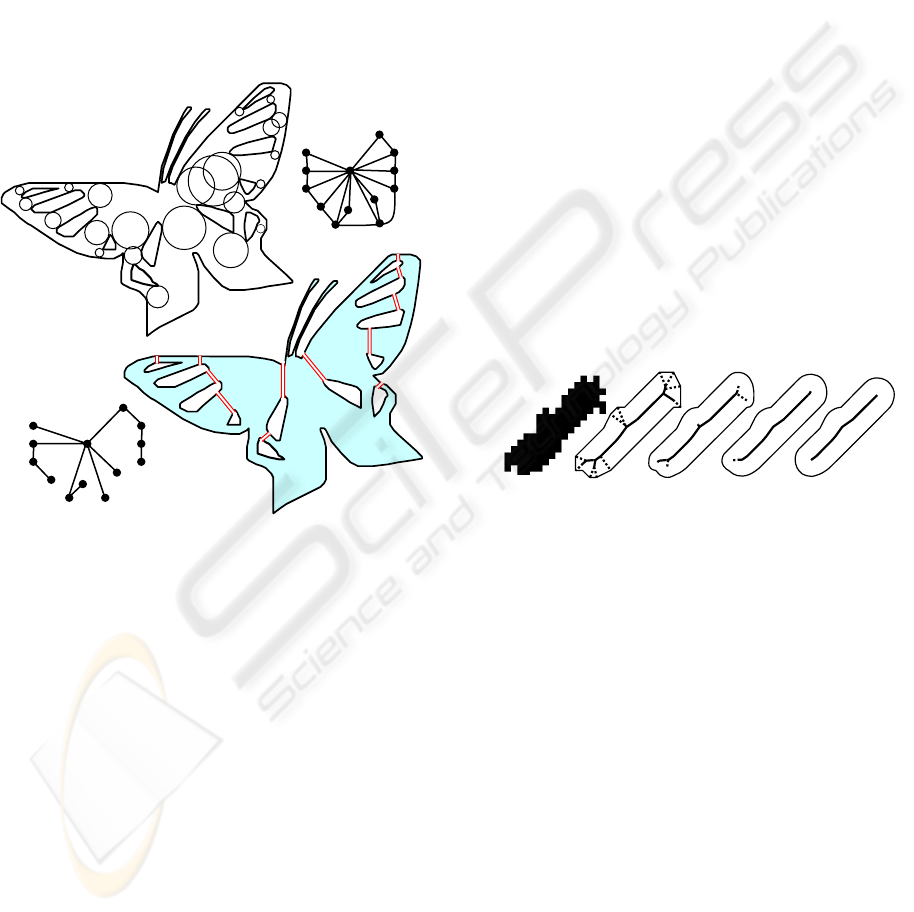
image (Mestetskiy, 2006) values k and n have an
order 10
3
and 10
5
accordingly. At the same time,
efficient algorithms for Voronoi diagram
construction of linear segment set (Fortune, 1987;
Yap, 1987) don’t use specific features of segment set
of polygonal figure boundary because of their
universality. In particular, these algorithms build
Voronoi partitioning not only inside, but also outside
of a polygonal figure and this is superfluous work.
Our solution is based on the concept of
adjacency of polygonal figure boundary contours
and on the construction of so-called adjacency tree
of these contours.
Figure 6: Figure boundary adjacency tree construction: (a)
the polygonal figure and intercontour circles, (b) the
boundary adjacency graph, (c) the boundary adjacency
tree, (d) transforming of the figure to the polygon.
Two boundary polygons are adjacent if the
circle inscribed into a figure, which contacts both of
these polygons exist. The given relation of contour
adjacency defines a graph of contour adjacency. It is
obvious, that this graph is connected. Each spanning
set of it (the minimal connected spanning subgraph)
is a tree. Such tree we will call a polygonal figure
boundary adjacency tree. In figure 6a the image with
12 boundary contours is presented. Inscribed circles,
contacting pairs of contours, show the adjacency
relation. In Fig.6(b) the polygonal figure boundary
adjacency is shown, and in Fig.6(c) one of the
boundary adjacency trees is presented.
The boundary adjacency tree gives the chance
to reduce a problem of a polygonal figure
skeletonization to a problem of a simple polygon
skeletonization. For this purpose let us transform
chains of polygon sides into one chain by «cutting-
in» them into one another. As a result the polygonal
figure conditionally transforms to "polygon"
(Fig.6(d)). An O (n log n) sweepline algorithm for
boundary adjacency tree finding and figure skeleton
construction is described in (Mestetskiy, 2006).
3.4 Skeletal Base
It is possible to present the process of a skeletal base
construction as a construction of a sequence of
truncated subgraphs of skeleton
{}
m
S
′
. Here
SS
=
′
0
,
mm
SS
′
⊂
′
+1
, m=0,…,M, and for all
m
S
′
the following condition is satisfied:
ε
≤
′
),(
m
S
VCH . The last element of this sequence
M
S
′
is the required skeletal base. According to our
definition of a skeletal base, for each truncated
subgraph
M
SS
′
⊂
′
condition
ε
>
′
),(
S
VCH
takes place or there are no terminal edges in
M
S
′
.
The described process is illustrated by an example in
Fig.7. Here
2
=
ε
.
Figure 7: Skeletal base construction: (a) the initial image,
(b) the polygonal figure and its skeleton, (c,d,e) the
skeleton subgraphs and their silhouettes.
Computational complexity of this algorithm
depends on the number of skeleton vertices linearly,
i.e. it is at worst O(n), where n is the number of
polygonal figure vertices.
4 EXPERIMENTS
The described method of continuous skeleton
construction of a binary image has been
implemented and has passed multiple checks in
different applications.
Theoretical estimates of computational complexity
of algorithms, with all their importance, don’t give
full conception about the possible application of
algorithms in computer vision systems. Therefore
there is a necessity to perform
(
a
)
(
b
)
(
c
)
(
d
)
(
e
)
(c)
(d)
(a)
(b)
0
1
2
3
4
5
6
7
8
9
10
11
12
1
2
11
10
9
8
7
4
3
0
12
6 5
6
5
10
1
2
11
9
7
3
0
12
8
VISAPP 2008 - International Conference on Computer Vision Theory and Applications
256
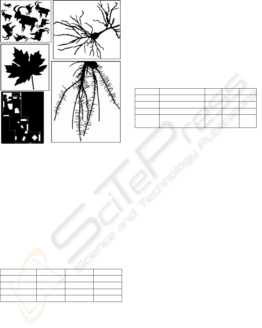
Figure 8: Test examples: (a) Billygoat, (b) leaf1, (c) room,
(d) neuron, (e) roots.
experimental estimates based on real working
algorithms and on practical examples. There is not
many publications describing such experiments.
Usually there is no information about software
implementation and algorithm running time at all
(Manzanera et al., 1999) or there are only results of
computing experiments with "toy" examples of very
simple images (Deng et al., 2000).
The most difficult examples (Fig.8) of images
and real time expenses for their skeletonization are
presented in works (Ogniewicz and Kubler, 1995;
Strzodka and Telea, 2004).
Table 1: Comparison of our algorithm CS and algorithm
OK (Ogniewicz and Kubler, 1995).
OK CS OK/CS
sites
11104 1874
5.92
edges 31381 3721 8.43
vertices 20303 3730 5.44
time 9.82 0.05 196.4
Results of comparison of our algorithm with the
algorithms described in these works, are given in
tables 1 and 2. Quality of the derived continuous
skeletons is shown on examples in Fig. 9, 10.
The running time of our algorithm was
estimated using Intel processor 1.6 GHertz with 512
Mb of memory. Time in tables is specified in
seconds.
Comparison with algorithm (Ogniewicz,
Kubler, 1995) shows, that using MPP for image
boundary approximation allows to reduce dimension
of the problem substantially: number of elements in
a polygonal figure skeleton is about 6-8 times less
than in a corresponding Voronoi diagram of image
boundary points. The reduction in computation time
(in 196 times) is partially due to this dimension
reduction, and partially due to processors capacity
increase as compared with SPARCstation-2.
Table 2: Comparison of our algorithm CS and algorithm
ST (Strzodka and Telea, 2004).
Size ST CS ST/CS
Leaf1 410×440=182040 0.14 0.02 70
Room 413×506=208978 0.64 0.03 21
Neuron 839×731=613309 2.5 0.1 25
Roots 1800×1810=
3258000
3.79 0.41 9.22
A new parallel discrete skeletonization algorithm
is described in Strzodka and Telea (2004). Authors
show that the running time of this algorithm is a
record for discrete algorithms so far. The table
shows the results attained by the authors on GPU
GeForce FX 5800 Ultra chip, containing tens
independent computers working in a parallel mode.
However, it is apparent from table 2, the running
time of our algorithm is less than of that algorithm
by 1-2 orders. It is necessary to note, that our
algorithm can be parallelized too and its operation
speed on multicore processors will grow.
5 CONCLUSIONS
The continuous approach to image skeleton
construction exceeds in many criteria traditionally
applied discrete methods.
1. The continuous skeleton is described by the
strict mathematical model. The discrete skeleton
doesn’t have such strict description; it is validated
only as an analogue of a continuous skeleton.
2. Regularization of continuous skeletons,
directed on noise overcoming, can be performed by
strict mathematical methods; and as for discrete
skeletons, it is done on the basis of heuristic devises.
3. The continuous skeleton with the radius
function gives more ample opportunities on shape
transformations of an object. Comparison of
continuous skeletons is reduced to a problem of
planar graphs comparison by topological and metric
criteria.
(a)
(e)
(b)
(c)
(d)
BINARY IMAGE SKELETON - Continuous Approach
257
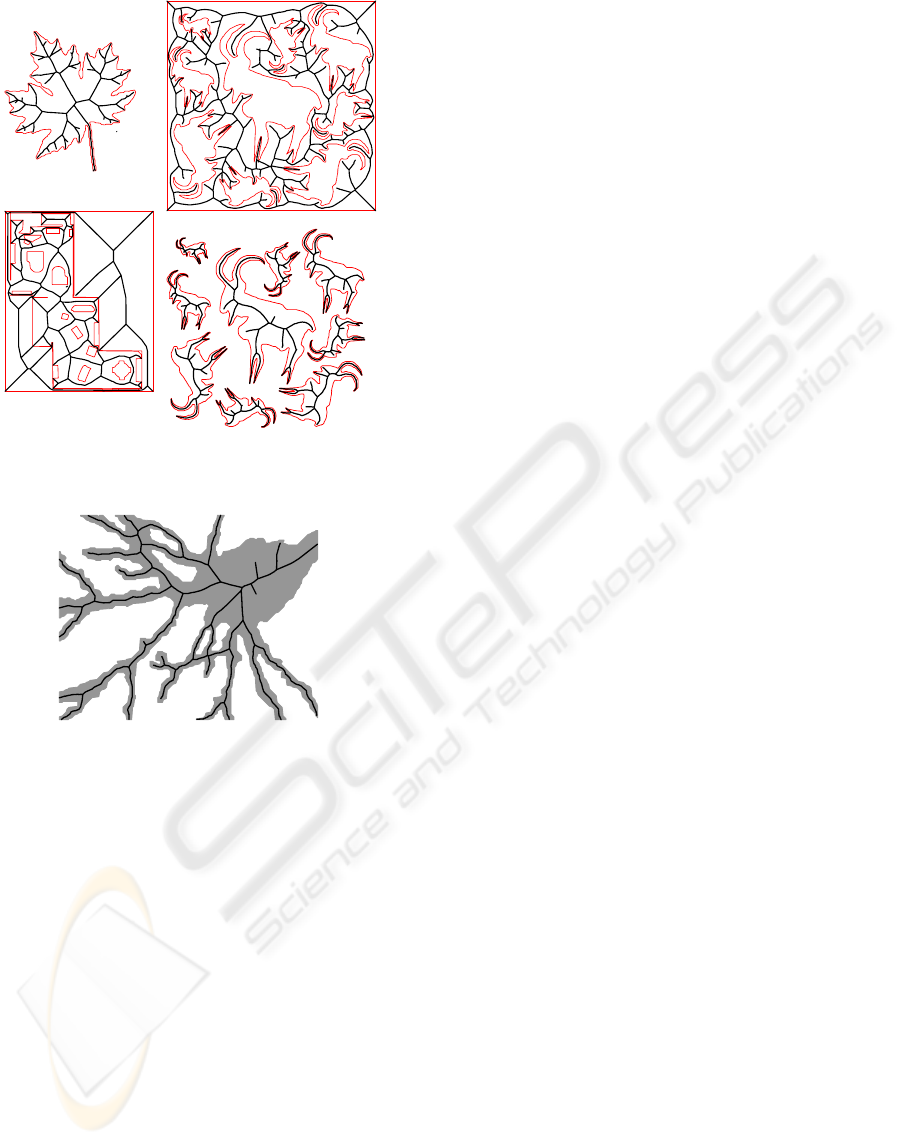
Figure 9: Continuous skeletons: (a) leaf1, (b) room,
(c) Billygoat (external), (d) Billygoat (internal).
Figure 10: The fragment of the skeleton for “neuron”.
4. Running time of continuous skeletonization
algorithm is less by at least an order than that of the
best samples of discrete skeletonization algorithms.
The downside of application of continuous
skeleton construction algorithm is the complexity of
its software implementation which demands rather
refined programming technique.
ACKNOWLEDGEMENTS
The authors thank Dr. R.Strzodka who has granted
us image samples for experiments. Also authors are
grateful to the Russian Foundation of Basic
Research, which has supported this work (grant 05-
01-00542).
REFERENCES
Bai, X., Latecki, L.J., Liu, W.-Y, 2007. Skeleton pruning
by contour partitioning with discrete curve evolution.
IEEE transactions on pattern analysis and machine
intelligence, vol. 29, No. 3, March 2007.
Blum, H., 1967. A transformation for extracting new
descriptors of shape. In Proc. Symposium Models for
the perception of speech and visual form, MIT Press
Cambridge MA, 1967.
Costa, L., Cesar, R., 2001. Shape analysis and
classification, CRC Press.
Deng, W., Iyengar, S., Brener, N., 2000. A fast parallel
thinning algorithm for the binary image
skeletonization. The International Journal of High
Performance Computing Applications, 14, No. 1,
Spring 2000, pp. 65-81.
Fortune S., 1987. A sweepline algorithm for Voronoi
diagrams. Algorithmica, 2 (1987), pp. 153-174.
Klein, R., Lingas, A., 1995. Fast skeleton construction. In
Proc. 3
rd
Europ. Symp. on Alg. (ESA’95), 1995.
Lagno, D., Sobolev, A., 2001. Модифицированные
алгоритмы Форчуна и Ли скелетизации
многоугольной фигуры. In Graphicon’2001,
International Conference on computer graphics,
Moscow, 2001 (in Russian).
Lee, D., 1982. Medial axis transformation of a planar
shape. IEEE Trans. Pat. Anal. Mach. Int. PAMI-4(4):
363-369, 1982.
Manzanera, A., Bernard, T., Preteux, F., Longuet, B.,
1999. Ultra-fast skeleton based on an isotropic fully
parallel algorithm. Proc. of Discrete Geometry for
Computer Imagery, 1999.
Mestetskiy, L., 1998. Continuous skeleton of binary raster
bitmap. In Graphicon’98, International Conference on
computer graphics, Moscow, 1998 (in Russian).
Mestetskiy, L., 2000. Fat curves and representation of
planar figures. Computers & Graphics, vol.24, No. 1,
2000, pp.9-21.
Mestetskiy, L., 2006. Skeletonization of a multiply
connected polygonal domain based on its boundary
adjacent tree. In Siberian journal of numerical
mathematics, vol.9, N 3, 2006, 299-314, (in Russian).
Ogniewicz, R., Kubler, O., 1995. Hierarchic Voronoi
Skeletons. Pattern Recognition, vol. 28, no. 3, pp.
343-359, 1995.
Smith R., 1987. Computer processing of line images: A
survey. Pattern recognition, vol. 20, no.1, pp.7-15,
1987.
Srinivasan, V., Nackman, L., Tang, J., Meshkat, S., 1992.
Automatic mesh generation using the symmetric axis
transform of polygonal domains, Proc. of the IEEE, 80
(9) (1992), pp. 1485–1501.
Strzodka, R., Telea, A., 2004. Generalized Distance
Transforms and Skeletons in Graphics Hardware. Joint
EUROGRAPHICS – IEEE TCVG Symposium on
Visualization (2004).
Yap C., 1987. An O(n log n) algorithm for the Voronoi
diagram of the set of simple curve segments. Discrete
Comput. Geom., 2(1987), pp. 365-393.
(a)
(b)
(c)
(d)
VISAPP 2008 - International Conference on Computer Vision Theory and Applications
258
