
EXPERIMENTAL EVALUATION OF RELATIVE POSE
ESTIMATION ALGORITHMS
Marcel Brückner, Ferid Bajramovic and Joachim Denzler
Chair for Computer Vision, Friedrich-Schiller-University Jena, Ernst-Abbe-Platz 2, 07743 Jena, Germany
Keywords:
Relative pose, epipolar geometry, camera calibration.
Abstract:
We give an extensive experimental comparison of four popular relative pose (epipolar geometry) estimation
algorithms: the eight, seven, six and five point algorithms. We focus on the practically important case that only
a single solution may be returned by automatically selecting one of the solution candidates, and investigate the
choice of error measure for the selection. We show that the five point algorithm gives very good results with
automatic selection. As sometimes the eight point algorithm is better, we propose a combination algorithm
which selects from the solutions of both algorithms and thus combines their strengths. We further investigate
the behavior in the presence of outliers by using adaptive RANSAC, and give practical recommendations for
the choice of the RANSAC parameters. Finally, we verify the simulation results on real data.
1 INTRODUCTION
Solving the relative pose problem is an important pre-
requisite for many computer vision and photogram-
metry tasks, like stereo vision. It consists of estimat-
ing the relative position and orientation of two cam-
eras from inter-image point correspondences, and is
closely related to the epipolar geometry. It is gener-
ally agreed, that bundle adjustment gives the best so-
lution to the problem (Triggs et al., 1999), but needs
a good initial solution for its local optimization.
In this paper, we review and experimentally
compare four non-local algorithms for estimating
the essential matrix and thus relative pose, which
can be used to initialize bundle adjustment: vari-
ants of the eight point and seven point algorithms
(Hartley and Zisserman, 2003), which directly esti-
mate the essential matrix, as well as a simple six
point algorithm and the five point algorithm, which
has been proposed recently (Stewénius et al., 2006).
In contrast to the experiments presented there, we
add an automatic selection of the best of the multiple
solutions computed by the five and seven point algo-
rithms, as it seems practically more relevant to get ex-
actly one solution. We also analyse the choice of the
epipolar error measure required by the selection step.
As there is no single best algorithm, we propose
the improvement of combining the best two algo-
rithms followed by a selection step. To the best of
our knowledge, this is a novel contribution.
Practically, point correspondences, which have
been automatically extracted from images, always
contain false matches. Estimating relative pose from
such data requires a robust algorithm. The RANSAC
scheme (Fischler and Bolles, 1981) gives robust vari-
ants of the algorithms mentioned above. In this pa-
per, we analyse the optimal choice of the error mea-
sure, the threshold and the sample size for RANSAC,
and give practical recommendations. We also investi-
gate the improvement gained by our combination al-
gorithm. Finally, we present results on real data.
The paper is structured as follows: In section 2,
we give a repetition of important theoretical basics
followed by a description of the algorithms in sec-
tion 3. We present our experiments in section 4 and
give conclusions in section 5.
2 THEORY
In this section, we introduce the camera model
and some notation and give a short repetition
of theoretical basics of the relative pose prob-
lem. For further details, the reader is referred to
(Hartley and Zisserman, 2003).
2.1 Camera Model
The pinhole camera model is expressed by the
equation p Kp
C
, where p
C
is a 3D point in
431
Brückner M., Bajramovic F. and Denzler J. (2008).
EXPERIMENTAL EVALUATION OF RELATIVE POSE ESTIMATION ALGORITHMS.
In Proceedings of the Third International Conference on Computer Vision Theory and Applications, pages 431-438
DOI: 10.5220/0001073704310438
Copyright
c
SciTePress

the camera coordinate system, p = (p
x
, p
y
, 1)
T
is
the imaged point in homogeneous 2D pixel coor-
dinates, denotes equality up to scale and K
def
=
((f
x
, s, o
x
), (0, f
y
, o
y
), (0, 0, 1))
T
is the camera calibra-
tion matrix, where f
x
and f
y
are the effective focal
lengths, s is the skew parameter and (o
x
, o
y
) is the
principal point. The relation between a 3D point in
camera coordinates p
C
and the same point expressed
in world coordinates p
W
is p
C
= Rp
W
+ t, where R is
the orientation of the camera and t defines the posi-
tion of its optical center. Thus, p
W
is mapped to the
image point p by the equation p K(Rp
W
+ t). We
will denote a pinhole camera by the tuple (K, R, t).
2.2 Relative Pose
The relative pose (R, t) of two cameras (K, I, 0),
(K
′
, R, t) is directly related to the essential matrix E:
E
def
[t]
×
R , (1)
where [t]
×
denotes the skew symmetric matrix asso-
ciated with t. The relative pose (R, t) can be recov-
ered from E up to the scale of t and a four-fold am-
biguity, which can be resolved by the cheirality con-
straint. The translation t spans the left nullspace of E
and can be computed via singular value decomposi-
tion (SVD).
The essential matrix is closely related to the fun-
damental matrix which can be defined as:
F
def
K
−T
EK
′
−1
. (2)
The matrices F and E fulfill the following properties:
p
T
Fp
′
= 0 (3)
ˆp
T
Eˆp
′
= 0 , (4)
where p and p
′
are corresponding points in the two
cameras (i.e. images of the same 3D point), and ˆp =
K
−1
p denotes camera normalized coordinates. Fur-
thermore, both matrices are singular:
det(F) = 0 and det(E) = 0 . (5)
The essential matrix has the following additional
property (Nistér, 2004), which is closely related to the
fact, that its two non-zero singular values are equal:
EE
T
E−
1
2
trace
EE
T
E = 0 . (6)
3 ALGORITHMS
3.1 Eight Point Algorithm
The well known eight point algorithm estimates F
from at least eight point correspondences based on
equation (3). According to equation (2), E can be
computed from F. As equation (4) has the same struc-
ture as (3), the (identical) eight point algorithm can
also be used to directly estimate E from camera nor-
malized point correspondences (ˆp, ˆp
′
).
Equation (4) can be written as ˜a
T
˜e = 0, with
˜a
def
=
ˆp
′
1
ˆp
1
, ˆp
′
2
ˆp
1
, ˆp
′
3
ˆp
1
, ˆp
′
1
ˆp
2
, ˆp
′
2
ˆp
2
, ˆp
′
3
ˆp
2
, ˆp
′
1
ˆp
3
, ˆp
′
2
ˆp
3
, ˆp
′
3
ˆp
3
T
(7)
˜e
def
=
(
E
11
,E
12
,E
13
,E
21
,E
22
,E
23
,E
31
,E
32
,E
33
)
T
. (8)
Given n ≥ 8 camera normalized point correspon-
dences, the according vectors a
T
i
can be stacked into
an n × 9 data matrix A with A˜e = 0. For n = 8, A
has rank defect 1 and ˜e is in its right nullspace. Let
A = Udiag(s)V
T
be the singular value decomposition
(SVD) of A. Troughout the paper, the singular val-
ues are assumed in decreasing order in s. Then ˜e is
the last column of V. For n > 8, this gives the least
squares approximation with k˜ek = 1.
3.2 Seven Point Algorithm
The seven point algorithm is very similar to the eight
point algorithm, but additionally uses and enforces
equation (5). It thus needs only seven point corre-
spondences. As in the eight point algorithm, the SVD
of the data matrix A is computed. For n = 7, A has
rank defect 2, and ˜e is in its two dimensional right
nullspace, which is spanned by the last two columns
of V. These two vectors are transformed back into the
matrices Z and W according to equation (8). We get:
E = zZ + wW , (9)
where z, w are unknown real values. Given the ar-
bitrary scale of E, we can set w = 1. To compute
z, substitute equation (9) into equation (5). This re-
sults in a third degree polynomial in z. Each of the
up to three real roots gives a solution for E. We use
the companion matrix method to compute the roots
(Cox et al., 2005). In case of n > 7, the algorithm is
identical. The computation of the nullspace is a least
squares approximation.
3.3 Six Point Algorithm
There are various six point algorithms (Philip, 1996;
Pizarro et al., 2003). Here, we present a simple one.
For n = 6, the data matrix has rank defect 3, and ˜e
is in its three dimensional right nullspace, which is
spanned by the last three columns of V. These three
vectors are transformed back into the matrices Y, Z
and W according to equation (8). Then we have:
E = yY + zZ + wW , (10)
VISAPP 2008 - International Conference on Computer Vision Theory and Applications
432

where y, z, w are unknown real values. Given the ar-
bitrary scale of E, we can set w = 1. To compute y
and z, substitute equation (10) into equation (6). This
results in nine third degree polynomials in y and z:
Bv = 0, v
def
=
y
3
, y
2
z,yz
2
, z
3
, y
2
, yz,z
2
, y, z,1
T
, (11)
where the 9× 10 matrix B contains the coefficients of
the polynomials. The common root (y, z) of the nine
multivariate polynomials can be computed by various
methods. As the solution is unique, we can choose
a very simple method: compute the right nullvector
b of B via SVD and extract the root y = b
8
/b
10
, z =
b
9
/b
10
. Note, however, that this method ignores the
structure of the vector v. According to equation (10),
this finally gives E. For n > 6, the same algorithm can
be applied.
3.4 Five Point Algorithm
The first part of the five point algorithm is very similar
to the six point algorithm. For n= 5, A has rank defect
4 and we get the following linear combination for E:
E = xX + yY + zZ + wW , (12)
where x, y, z, w are unknown scalars and X, Y, Z,W are
formed from the last four columns of V according
to equation (8). Again, we set w = 1. Substituting
equation (12) into the equations (5) and (6) gives ten
third degree polynomials Mm= 0 in three unknowns,
where the 10× 20 matrix M contains the coefficients
and the vector m contains the monomials:
m =
(
x
3
,x
2
y,x
2
z,xy
2
,xyz,xz
2
,y
3
,y
2
z,yz
2
,z
3
,x
2
,xy,xz,y
2
,yz,z
2
,x,y,z,1
)
T
.
The multivariate problem can be transformed
into a univariate problem, which can then be
solved using the companion matrix or Sturm se-
quences (Nistér, 2004). A more efficient vari-
ant of the five point algorithm (Stewénius, 2005;
Stewénius et al., 2006) directly solves the multivari-
ate problem by using Gröbner bases. First, Gauss Jor-
dan elimination with partial pivotization is applied to
M. This results in a matrix M
′
= (I|B), where I is
the 10× 10 identity matrix and B is a 10 × 10 matrix.
The ten polynomials defined by M
′
are a Gröbner ba-
sis and have the same common roots as the original
system. Now, form the 10× 10 action matrix C as fol-
lows: the first six rows of C
T
equal the first six rows of
B, C
1,7
= 1, C
2,8
= 1, C
3,9
= 1, C
7,10
= 1, all remaining
elements are zero. The eigenvectors u
i
corresponding
to real eigenvalues of C
T
give the up to ten common
real roots: x
i
= u
i,7
/u
i,10
, y
i
= u
i,8
/u
i,10
, z
i
= u
i,9
/u
i,10
.
By substituting into equation (12), each root (x
i
, y
i
, z
i
)
gives a solution for E.
3.5 Normalization
According to (Hartley and Zisserman, 2003), point
correspondences should be normalized before apply-
ing the eight or seven point algorithm to improve sta-
bility. The (inhomogeneous) points are normalized
by translating such that their mean is in the origin and
scaling by the inverse of their average norm. In homo-
geneous coordinates, the third coordinate (assumed to
be 1 for all points) is simply ignored and not changed.
The normalization is applied in each image indepen-
dently. When using camera normalized coordinates,
the same normalization can be used. For the six and
five point algorithms, however, such a normalization
is not possible, as it does not preserve equation (6).
3.6 Constraint Enforcement
Note that the solution computed by the eight and
seven point algorithms does not respect all proper-
ties of an essential matrix as presented in section 2.2.
This might also be the case for the six point algo-
rithm because of the trick applied to solve the polyno-
mial equations (ignoring the structure of the vector v).
Thus, each resulting essential matrix should be cor-
rected by enforcing that its singular values are (s, s, 0)
with s > 0 (we use s = 1). This can be achieved by
SVD and subsequent matrix multiplication using the
desired singular values.
Even though the five point algorithm actually
computes valid essential matrices, we also apply the
constraint enforcement to them. This has the addi-
tional effect of normalizing the scale of the essential
matrices, which appears desireable for some of the
experiments.
3.7 Selecting the Correct Solution
The seven and five point algorithms can produce more
than one solution. If there are additional point cor-
respondences, the single correct solution can be se-
lected. For each solution, the deviation of each cor-
respondence from the epipolar constraint is measured
and summed up over all correspondences. The solu-
tion with the smallest error is selected. There are var-
ious possibilities to measure the deviation from the
epipolar constraint (Hartley and Zisserman, 2003):
1. The algebraic error:
p
T
Fp
′
.
2. The symmetric squared geometric error:
p
T
Fp
′
2
Fp
′
2
1
+
Fp
′
2
2
+
p
T
Fp
′
2
h
F
T
p
i
2
1
+
h
F
T
p
i
2
2
, (13)
where [·]
i
denotes the ith element of a vector,
EXPERIMENTAL EVALUATION OF RELATIVE POSE ESTIMATION ALGORITHMS
433
3. The squared reprojection error d
2
(
p, q
)
2
+
d
2
(
p
′
, q
′
)
2
, where d
2
denotes the Euclidean
distance, and q and q
′
are the reprojections
of the triangulated 3D point. For a suitable
triangulation algorithm, the reader is referred
to the literature (Hartley and Sturm, 1997;
Hartley and Zisserman, 2003).
4. The Sampson error:
p
T
Fp
′
2
Fp
′
2
1
+
Fp
′
2
2
+
h
F
T
p
i
2
1
+
h
F
T
p
i
2
2
. (14)
3.8 RANSAC
To achieve robustness to false correspondences, the
well known (adaptive) RANdom SAmple Concen-
sus (RANSAC) algorithm (Fischler and Bolles, 1981;
Hartley and Zisserman, 2003) can be applied:
Input: Point correspondences D.
1. Iterate k times:
(a) Randomly select m elements from D.
(b) Estimate the essential matrix from this subset.
(c) For each resulting solution E:
i. Compute S = { (p, p
′
) ∈ D | d
E
(p, p
′
) < c},
where d
E
is an error measure from section 3.7.
ii. If S is larger than B: set B := S and adapt k.
2. Estimate E from B with automatic selection of the
correct solution.
For details, the reader is referred to the literature. We
will investigate the choice of the parameters m and c.
3.9 Combining Algorithms
There is no single best algorithm for all situations.
This makes it difficult to choose a single one, espe-
cially if there is no prior knowledge about the cam-
era motion (see section 4). Hence, we propose the
novel approach of combining two or more algorithms,
which exploits their combined strengths. We run sev-
eral algorithms on the same data to produce a set of
candidate solutions. The automatic selection proce-
dure is applied to select the best solution. We call this
procedure the combination algorithm.
It is straight forward to apply the combination in
RANSAC. However, we also have the possibility to
use a single algorithm during RANSAC iterations and
a combination for the final estimation from the best
support set B. We will use the name final combina-
tion for this strategy. It has the advantage that the
five point algorithm can be used during iterations with
small sample size m = 5 and the five and eight point
algorithms can be combined for the final estimation.
[e
T
]
80
70
60
50
40
30
20
10
0
[n]45403530252015105
geometric, 5 point
reprojection, 5 point
Sampson, 5 point
algebraic, 5 point
ideal, 5 point
geometric, combi
reprojection, combi
Sampson, combi
algebraic, combi
ideal, combi
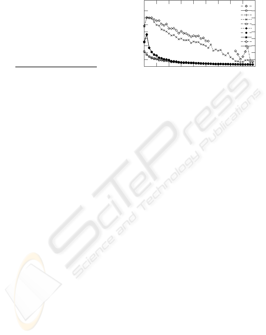
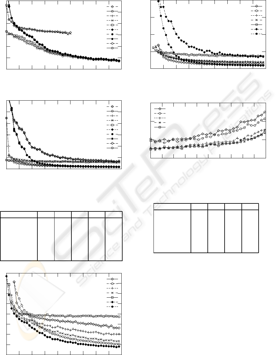
Figure 1: Comparison of error measures for automatic se-
lection of the best solution in the five point algorithm, side-
ways motion. Median translation error e
T
for varying num-
ber of point correspondences n. The plots for “euclidean”,
“reprojection”, “Sampson” and their “combi” variants are
almost identical, as are “ideal” and “ideal, combi”.
4 EXPERIMENTS
4.1 Simulation
The simulation consists of two virtual pinhole cam-
eras (K, I, 0) and (K, R
G
, t
G
) with image size 640 ×
480, f
x
= f
y
= 500, s = 0, o
x
= 320, o
y
= 240. The
scene consists of random 3D points uniformly dis-
tributed in a cuboid (distance from first camera 1,
depth 2, width and height 0.85). These 3D points
can be projected into the cameras. Noise is simu-
lated by adding random values uniformly distributed
in [−φ/2, φ/2] to all coordinates. We choose φ = 3 for
all experiments.
We use two different error measures to compare
the estimate for E to the ground truth for relative pose:
• The translation error e
t
is measured by the angle
(in degree, 0 ≤ e
t
≤ 90) between the ground truth
translation t
G
and the estimate computed from E.
• The rotation error e
r
is measured by the rota-
tion angle (in degree, 0 ≤ e
r
≤ 180) of the rela-
tive rotation R
rel
between the ground truth orien-
tation R
G
and the estimate R
E
computed from E:
R
rel
= R
G
R
T
E
. The ambiguity resulting in two so-
lution for R
E
is resolved by computing the angle
for both and taking the smaller one as error e
r
.
All experiments are repeated at least 500 times each.
Finally, the median e
T
of e
t
and e
R
of e
r
over all rep-
etitions is computed. In the evaluation, we focus on
the median translation error e
T
and include results for
the median rotation error e
R
in the appendix. The ro-
tation error e
R
is much lower and gives structurally
very similar results.
VISAPP 2008 - International Conference on Computer Vision Theory and Applications
434
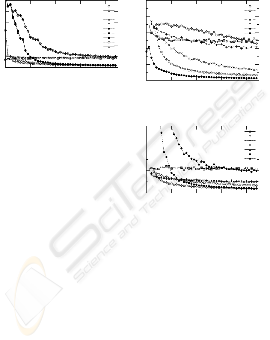
[e
T
]
50
40
30
20
10
0
[n]45403530252015105
geometric, 5 point
reprojection, 5 point
Sampson, 5 point
algebraic, 5 point
ideal, 5 point
geometric, combi
reprojection, combi
Sampson, combi
algebraic, combi
ideal, combi
Figure 2: Comparison of error measures for automatic se-
lection of the best solution in the five point algorithm, for-
ward motion. Median translation error e
T
for varying num-
ber of point correspondences n. The plots for “euclidean”,
“reprojection” and “Sampson” are almost identical, as are
their “combi” variants.
4.1.1 Outlier-free Data
First, we analyse the performance of the automatic
selection of the best solution for the five point algo-
rithm. Figure 1 shows the results for sideways mo-
tion (t
G
= (0.1, 0, 0)
T
, R
G
= I). It also contains the er-
ror of the ideal selection which is computed by com-
paring all essential matrices to the ground truth. The
automatic selection works equally well with all error
measures except for the algebraic one. Given enough
points, the results almost reach the ideal selection.
In case of forward motion (t
G
= (0, 0, −0.1)
T
, R
G
=
I), the algebraic error is best (figure 2). Given enough
points, the other error measures also givegood results.
For few points, however, the selection does not work
well. Thus, if there is no prior knowledge about the
translation, the Sampson or geometric error measure
are the most reasonable choice. The reprojection error
is also fine, but computationally more expensive.
The next experiment compares the various estima-
tion algorithms. In contrast to the results presented by
Stewénius, Engels and Nistér (Stewénius et al., 2006;
Nistér, 2004), we apply automatic selection with the
Sampson error measure for the five and seven point
algorithms, which gives a more realistic comparison.
Figures 3 and 4 show the results for sideways and
forward motion, respectively. For sideways motion,
the five point algorithm with automatic selection still
gives superior results. For forward motion, however,
the eight point algorithm is best. Surprisingly, in this
case, the eight point algorithm with data normaliza-
tion is worse than without normalization.
Given this situation, we add a combination of
the five point and the unnormalized eight point al-
gorithms to the comparison (“combi”). For sideways
motion (figures 1 and 3), the results of the combina-
[e
T
]
80
60
40
20
0
[n]45403530252015105
8 point
8 point norm.
7 point
7 point norm.
6 point
5 point
combi
Figure 3: Comparison of algorithms with Sampson error for
automatic selection, sideways motion. Median translation
error e
T
for varying number of point correspondences n.
The plots for “5 point” and “combi” are almost identical.
[e
T
]
20
10
0
[n]45403530252015105
8 point
8 point norm.
7 point
7 point norm.
6 point
5 point
combi
Figure 4: Comparison of algorithms, forward motion. Me-
dian translation error e
T
for varying number of point corre-
spondences n. The plots for “7 point” and “7 point norm.”
are mostly identical.
tion are almost identical to the five point results (ex-
cept for selection with the algebraic error). For for-
ward motion (figures 2 and 4), the automatic selection
works better than with the five point algorithm alone,
but still needs enough points to produce good results.
Then, however, the combination reaches the results of
the unnormalized eight point algorithm, which is the
best single algorithm in this situation.
The consequence of the simulation results is that
our combination with the Sampson error measure for
automatic selection is the best choice for outlier-free
data without prior knowledge about the translation.
4.1.2 RANSAC
Next, we analyse the best choice of the threshold
c and also the choice of the error measure for the
RANSAC variant of the five point algorithm. In this
experiment, we use a different camera setup: t
G
=
(0.1, 0, 0.1)
T
and R
G
is a rotation about the y axis
EXPERIMENTAL EVALUATION OF RELATIVE POSE ESTIMATION ALGORITHMS
435
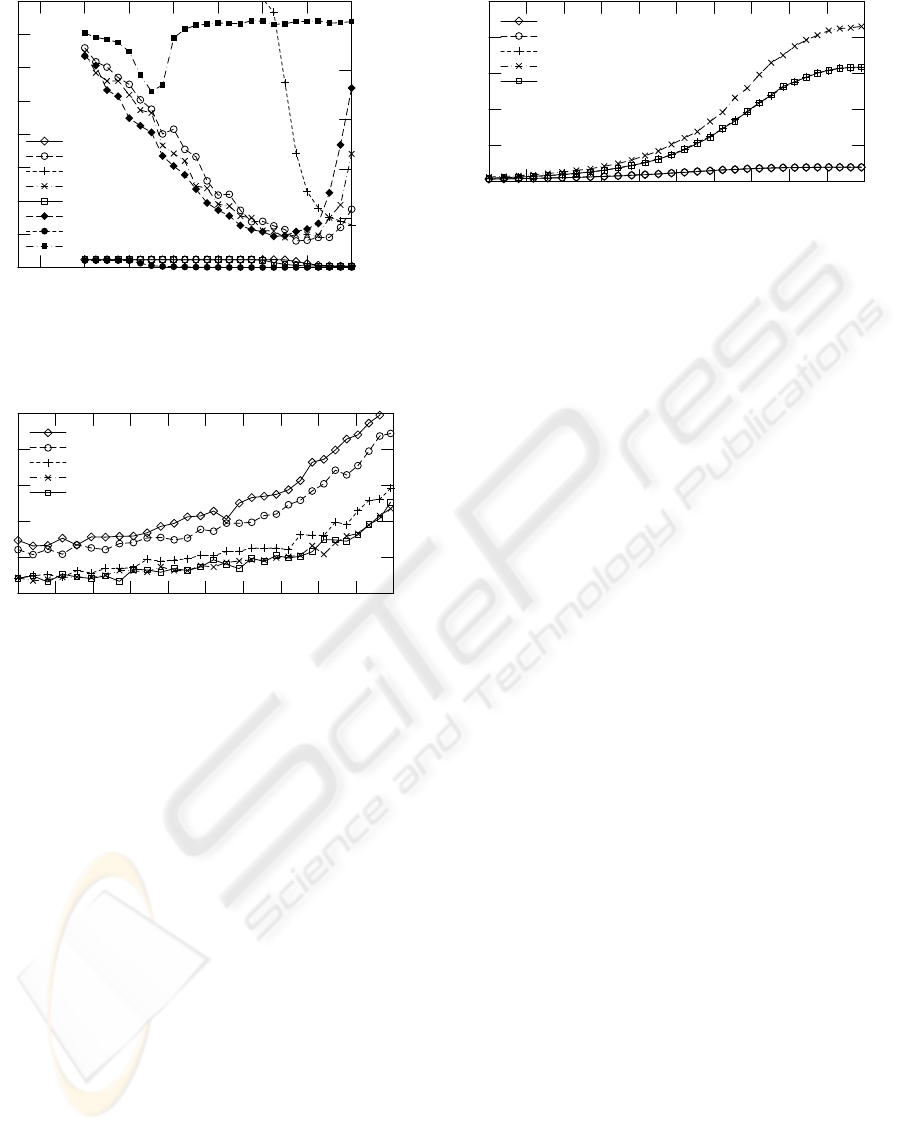
[e
T
]
40
35
30
25
20
15
10
5
[log
10
c]10-1-2-3-4
[t/s]
2.0
1.5
1.0
0.5
0
geometric, t
geometric, e
reprojection, t
reprojection, e
Sampson, t
Sampson, e
algebraic, t
algebraic, e
Figure 5: Five point RANSAC with all four error measures.
Median translation error e
T
and mean computation times
for varying values of the threshold c. Outlier probability
r = 29.44% (r
s.
= 16%).
[e
T
]
13
11
9
7
5
[r/%]454035302520151050
sample size 5, 5 point
sample size 5, final combi
sample size 8, 5 point
sample size 8, combi
sample size 8, final combi
Figure 6: Median translation error e
T
for RANSAC algo-
rithms with various sample sizes m on data with varying
amounts of outliers r.
by 0.01 (≈ 5.7
◦
). Outliers are generated by replac-
ing each projected image point by a randomly gener-
ated point within the image with probability r
s
. The
probability of a point pair being an outlier is thus
r = 1− (1− r
s
)
2
.
Figure 5 shows the median translation error as
well as the mean computation times for 29.44% out-
liers. The geometric, reprojection and Sampson error
measures give good results. However, the computa-
tion time for the reprojection error is at least 10 times
higher. Given an optimal threshold c
opt
, the geometric
error gives the best results, even though the difference
is small. However, as further experiments show, c
opt
depends on the amount of outliers r and is thus diffi-
cult to guess. For the Sampson error, c
opt
is much less
affected by r, and is roughly equal to the noise level.
In the next experiment, we analyse the choice of
the sample size m. We use the Sampson error with
threshold c = 1.5. Figure 6 shows that increasing the
sample size decreases the median translation error.
However, the computation time increases drastically
(figure 7). In case of sample size m = 8, we also in-
clude the combination of the five point and the unnor-
[t/s]
0.8
0.6
0.4
0.2
0
[r/%]454035302520151050
sample size 5, 5 point
sample size 5, final combi
sample size 8, 5 point
sample size 8, combi
sample size 8, final combi
Figure 7: Mean computation times for RANSAC algo-
rithms with various sample sizes m on data with varying
amounts of outliers r.
malized eight point algorithm (“combi”), which gives
better results than the five point algorithm, but also
further increases the computation time. Note, how-
ever, that the implementation could be optimized by
exploiting that the first part of both algorithms is iden-
tical (SVD of data matrix). For sample sizes m = 5
and m = 8, we apply the final combination algorithm
using the five point algorithm during RANSAC itera-
tions and the five point and unnormalized eight point
algorithms only for the final estimation from the best
support set (“final combi”). In case of m = 8, this
approach gives comparably good results to the previ-
ous case, but without the additional computation time.
Furthermore, we also get the final combination bene-
fit for sample size m = 5.
4.2 Real Data
To verify the results presented above, we also perform
experiments with a calibrated camera (Sony DFW-
VL500) mounted onto a robotic arm, which provides
us with ground truth data for relative pose. We record
two different sequences: motion on a sphere around
the scene in 10
◦
steps with the camera pointing to the
center (five image pairs), and forward motion (four
image pairs). The scenes are shown in figure 8. We
use SIFT (Lowe, 2004) to detect 200 point correspon-
dences. These are fed into the RANSAC variants (us-
ing the Sampson error with m = 8 and c = 1) of all
algorithms presented in section 3, and also the “final
combi” algorithm as in the synthetic experiments.
The results are shown in tables 1 and 2. On the
first scene, only the five point and the “final combi”
algorithms give good results, which may be caused
by the dominantly planar distribution of the SIFT fea-
tures (Nistér, 2004). On the second scene, most algo-
rithms work well. In contrast to the synthetic experi-
ments with forward motion, the eight point algorithm
with normalization is better than without. It gives the
best results for this scene. The five point algorithm
has problems with the second image pair, but “final
VISAPP 2008 - International Conference on Computer Vision Theory and Applications
436
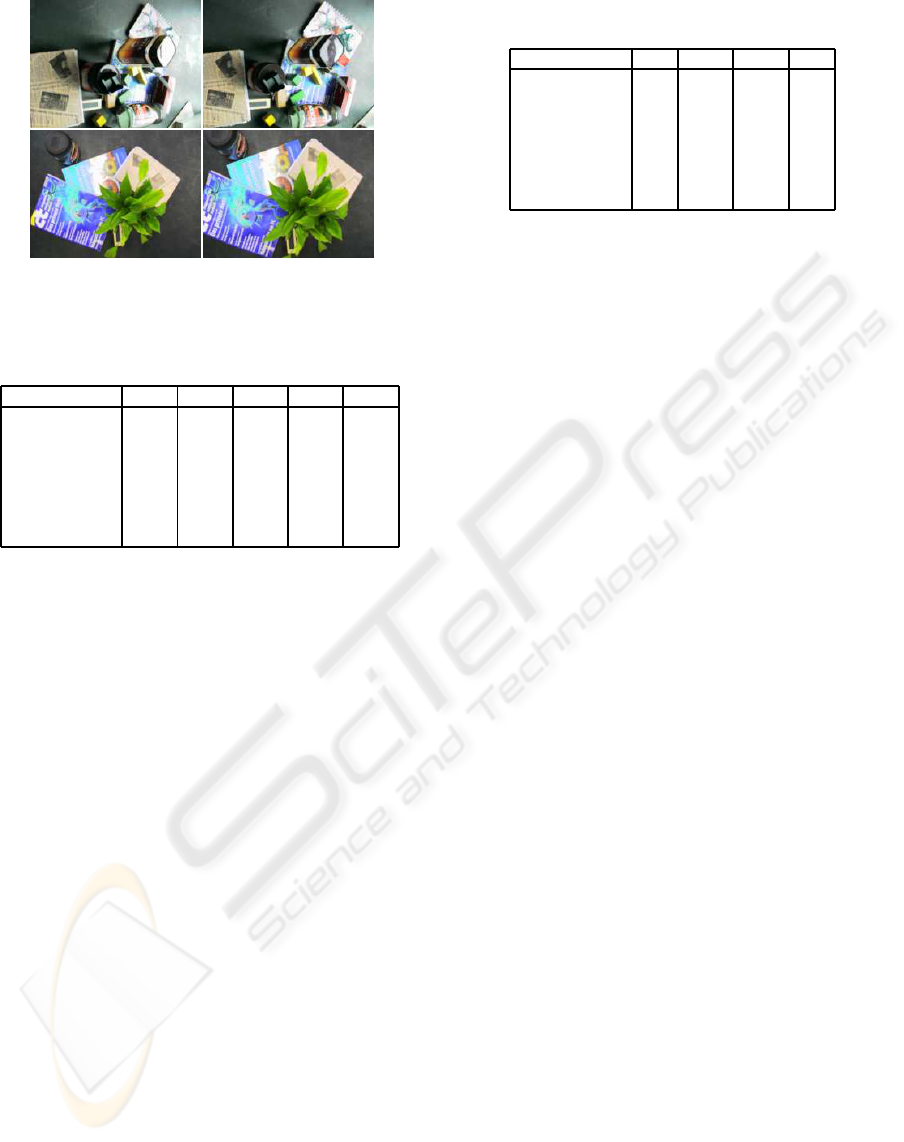
Figure 8: Scenes used for the experiments with real data.
Top: sequence 1, image pair 2. Bottom: sequence 2, pair 1.
Table 1: Median translation errors e
T
on scene 1.
image pair 1 2 3 4 5
5 point 0.8 1.9 0.7 0.4 1.0
final combi 0.8 1.9 0.7 0.4 1.0
6 point 40.0 61.3 65.1 26.9 4.9
7 point 59.0 62.6 69.0 2.4 2.0
7 point norm. 23.7 58.2 39.0 6.8 16.3
8 point 62.7 65.4 66.5 20.5 21.6
8 point norm. 65.9 36.0 29.9 6.6 15.4
combi” works well and is close to the eight point al-
gorithm. Overall, these experiments show that the “fi-
nal combi” algorithm is the best choice if there is no
prior knowledge about the relative pose.
5 CONCLUSIONS
We have shown that the five point algorithm with au-
tomatic selection of the single best solution gives very
good estimates for relative pose. Due to its prob-
lems with forward motion, we proposed a combina-
tion with the eight point algorithm and showed that
this gives very good results. In presence of outliers,
RANSAC provides the necessary robustness. Our (fi-
nal) combination is also beneficial in this case.
Finally, we summarize our recommendations for
cases without prior knowledge about the motion. We
suggest using RANSAC with the Sampson error, the
five point algorithm during iterations, and the five
point and normalized eight point algorithms for the
final estimation. We called this approach final com-
bination. The RANSAC threshold should be chosen
similar to the noise level. The sample size has to be
at least 5, but should be increased to 8 or 10 (or even
more) if computation time permits. Furthermore, it is
advantageous to use as many points as possible.
Table 2: Median translation errors e
T
on scene 2.
image pair 1 2 3 4
5 point 2.1 13.4 1.2 1.5
final combi 1.1 1.6 1.2 1.4
6 point 1.0 0.5 6.4 1.2
7 point 1.0 1.2 1.2 1.8
7 point norm. 5.9 17.8 13.0 2.7
8 point 1.2 1.7 1.4 1.6
8 point norm. 1.0 1.2 1.2 1.2
REFERENCES
Cox, D. A., Little, J., and O’Shea, D. (2005). Using Al-
gebraic Geometry. Graduate Texts in Mathematics.
Springer, 2nd edition.
Fischler, M. A. and Bolles, R. C. (1981). Random sam-
ple consensus: A paradigm for model fitting with ap-
plications to image analysis and automated cartogra-
phy. Communications of the Association for Comput-
ing Machinery, 24(6):381–395.
Hartley, R. and Sturm, P. (1997). Triangulation. Computer
Vision and Image Understanding, 68(2):146–157.
Hartley, R. and Zisserman, A. (2003). Multiple View Geom-
etry in Computer Vision. Cambridge University Press,
2nd edition.
Lowe, D. G. (2004). Distinctive image features from scale-
invariant keypoints. International Journal of Com-
puter Vision, 60(2):91–110.
Nistér, D. (2004). An efficient solution to the five-point
relative pose problem. IEEE Transactions on Pattern
Analysis and Machine Intelligence, 26(6):756–770.
Philip, J. (1996). A non-iterative algorithm for determining
all essential matrices corresponding to five point pairs.
Photogrammetric Record, 15(88):589–599.
Pizarro, O., Eustice, R., and Singh, H. (2003). Relative pose
estimation for instrumented, calibrated imaging plat-
forms. In Proceedings of Digital Image Computing
Techniques and Applications, pages 601–612.
Stewénius, H. (2005). Gröbner Basis Methods for Minimal
Problems in Computer Vision. PhD thesis, Centre for
Mathematical Sciences LTH, Lund Univ., Sweden.
Stewénius, H., Engels, C., and Nistér, D. (2006). Re-
cent Developments on Direct Relative Orientation. IS-
PRS Journal of Photogrammetry and Remote Sensing,
60(4):284–294.
Triggs, B., McLauchlan, P. F., Hartley, R. I., and Fitzgib-
bon, A. W. (1999). Bundle Adjustment — A Modern
Synthesis. In Proc. of the Int. Workshop on Vision Al-
gorithms: Theory and Practice, pages 298–373.
APPENDIX
In figures 9–13 and tables 3–4, we present additional
results for the rotation error e
R
. Each figure refers to
the corresponding figure for the translation error e
T
.
EXPERIMENTAL EVALUATION OF RELATIVE POSE ESTIMATION ALGORITHMS
437
[e
R
]
5
4
3
2
1
0
[n]45403530252015105
geometric, 5 point
reprojection, 5 point
Sampson, 5 point
algebraic, 5 point
ideal, 5 point
geometric, combi
reprojection, combi
Sampson, combi
algebraic, combi
ideal, combi
Figure 9: As figure 1, but using median rotation error e
R
.
[e
R
]
5
4
3
2
1
0
[n]45403530252015105
geometric, 5 point
reprojection, 5 point
Sampson, 5 point
algebraic, 5 point
ideal, 5 point
geometric, combi
reprojection, combi
Sampson, combi
algebraic, combi
ideal, combi
Figure 10: As figure 2, but using median rotation error e
R
.
Table 3: Median rotation errors e
R
on scene 1.
image pair 1 2 3 4 5
5 point 0.3 0.6 0.2 0.2 0.3
final combi 0.6 3.5 0.2 0.2 0.3
6 point 10.5 7.8 10.6 2.4 1.0
7 point 6.7 11.6 8.7 0.1 0.3
7 point norm. 8.8 8.8 10.1 9.9 20.0
8 point 12.7 11.7 11.1 3.1 8.8
8 point norm. 16.7 11.5 14.8 18.5 20.0
[e
R
]
7
6
5
4
3
2
1
0
[n]45403530252015105
8 point
8 point norm.
7 point
7 point norm.
6 point
5 point
combi
Figure 11: As figure 3, but using median rotation error e
R
.
[e
R
]
3
2
1
0
[n]45403530252015105
8 point
8 point norm.
7 point
7 point norm.
6 point
5 point
combi
Figure 12: As figure 4, but using median rotation error e
R
.
[e
R
]
1.5
1.0
0.5
[r/%]454035302520151050
sample size 5, 5 point
sample size 5, final combi
sample size 8, 5 point
sample size 8, combi
sample size 8, final combi
Figure 13: As figure 6, but using median rotation error e
R
.
Table 4: Median rotation errors e
R
on scene 2.
image pair 1 2 3 4
5 point 0.13 1.90 0.03 0.10
final combi 0.05 0.14 0.03 0.14
6 point 0.05 0.18 0.16 0.07
7 point 0.03 0.17 0.04 0.21
7 point norm. 0.23 3.04 0.56 0.89
8 point 0.05 0.12 0.04 0.12
8 point norm. 0.20 0.18 0.03 0.01
VISAPP 2008 - International Conference on Computer Vision Theory and Applications
438
