
A
NORMALIZED PARAMETRIC DOMAIN FOR THE ANALYSIS OF
THE LEFT VENTRICULAR FUNCTION
Jaume Garcia-Barnes, Debora Gil
Computer Vision Center, Campus UAB, Bellaterra, Spain
Sandra Pujadas, Francesc Carreras
Hospital de la Sta Creu i St Pau, Barcelona, Spain
Manel Ballester
Department of Cardiology, University of Lleida, Lleida, Spain
Keywords:
Helical Ventricular Myocardial Band, Myocardial Fiber, Tagged Magnetic Resonance, HARP, Optical Flow
Variational Framework, Gabor Filters, B-Splines.
Abstract:
Impairment of left ventricular (LV) contractility due to cardiovascular diseases is reflected in LV motion pat-
terns. The mechanics of any muscle strongly depends on the spatial orientation of its muscular fibers since
the motion that the muscle undergoes mainly takes place along the fiber. The helical ventricular myocardial
band (HVMB) concept describes the myocardial muscle as a unique muscular band that twists in space in a
non homogeneous fashion. The 3D anisotropy of the ventricular band fibers suggests a regional analysis of
the heart motion. Computation of normality models of such motion can help in the detection and localization
of any cardiac disorder. In this paper we introduce, for the first time, a normalized parametric domain that
allows comparison of the left ventricle motion across patients. We address, both, extraction of the LV motion
from Tagged Magnetic Resonance images, as well as, defining a mapping of the LV to a common normalized
domain. Extraction of normality motion patterns from 17 healthy volunteers shows the clinical potential of
our LV parametrization.
1 INTRODUCTION
The Helical Ventricular Myocardial Band (HVMB)
concept was developed during the last 50 years by Dr.
Torrent-Guasp after more than 1000 anatomical dis-
sections of hearts belonging to different species (Ko-
cica et al., 2006; Torrent-Guasp et al., 2005). His rev-
olutionary (though not fully accepted) theory states
that the architecture of the main cavities of the heart
arises from the disposition of a unique muscular band
in 3D space. This muscular band is twisted in two
helical loops from the root of the pulmonary artery to
the aorta.
Figure 1 shows the main dissection steps for ob-
taining the ventricular band of a bovine heart. Af-
ter unwrapping the myocardial band helical structure,
a single straight muscular band is obtained with the
pulmonary artery at one side and the aorta at the other
(Fig. 1.d). Over this band, four segments are distin-
guished: right segment (RS), left segment (LS), de-
scendent segment (DS) and ascendent segment (AS)
Figure
1: Main steps of the dissection of a bovine heart. In-
tact myocardium a), myocardial muscle showing the fibers
b), unwrapped myocardial band c) and the the four seg-
ments of the myocardial band d), which, from left to right,
are: right (RS), left (LS), descendent (DS) and ascendent
segments (AS). (Photos from (Kocica et al., 2006)).
267
Garcia-Barnes J., Gil D., Pujadas S., Carreras F. and Ballester M. (2008).
A NORMALIZED PARAMETRIC DOMAIN FOR THE ANALYSIS OF THE LEFT VENTRICULAR FUNCTION.
In Proceedings of the Third International Conference on Computer Vision Theory and Applications, pages 267-274
DOI: 10.5220/0001074002670274
Copyright
c
SciTePress

(Fig. 1.d). The complex spatial distribution of these
segments can be appreciated by coloring each of them
and wrapping the band again as illustrated in figure 2.
The longitudinal (left) and axial (right) views show
the complex disposition of the different segments in
the myocardium and reveal a highly anisotropic non
homogeneous tissue structure.
The contraction mechanics of any muscle strongly
depends on the spatial orientation of its muscular
fibers since the motion that the muscle undergoes
mainly takes place along the fiber (Waldman et al.,
1988). Any cardiovascular disease affecting the blood
supply at a given myocardial area affects the con-
tractile properties of the ventricular band and, thus,
the heart function. It follows that the function and
anatomy (given by the ventricular band) of the heart
are highly interdependent (Jung et al., 2006; Kocica
et al., 2006). The anisotropy in fiber orientation of
the ventricular band (fig.2) suggests a regional anal-
ysis of the heart motion rather than extracting global
scores, such as ejection fraction or wall thickening.
Currently, there are many medical imaging modal-
ities (echo-cardiography, magnetic resonance) that al-
low assessment of the heart function. Most of them
display the myocardium as an homogeneous tissue
so that only the outer (epicardium) and inner (endo-
cardium) border dynamics can be appreciated. Al-
though this suffices to compute global scores, extrac-
tion of tissue motion within the myocardial walls is
not feasible. The only technique that allows nonin-
vasive detailed visualization of the intra-myocardial
function is Tagged Magnetic Resonance (TMR) (Zer-
houni et al., 1988; Axel and Dougherty, 1989). This
technique prints a grid-like pattern of saturated mag-
netization over the myocardium, which, as it evolves
by the underlying motion of tissue, allows visualiza-
tion of intramural deformation.
Since the appearance of TMR many image pro-
cessing techniques have been developed in order to
obtain vector fields that reflect the functionality of the
heart. The techniques developed so far mainly fo-
cus on extracting local apparent physical scores (such
as strain (Garot et al., 2000; Gotte et al., 2006)) and
restoring 3D deformation from 2D TMR projections
in order to get more realistic measures of the heart in-
tegrity (Li and Denney, 2006; Luo and Heng, 2005).
However, few effort has been done towards the com-
putation of normality models for the ventricular func-
tion aimed at helping in the detection and localization
of cardiac disorders. Up to our knowledge, the only
authors addressing computation of motion models are
Rao (Rao et al., 2003) and Chandrashekara (Chan-
drashekara et al., 2003). Their models are designed
to add prior information for tracking algorithms and
Figure 2: Disposition of the main segments of the band in
space by coloring. A longitudinal cut is shown on the left
hand-side and two axial cuts from the basal (above) and api-
cal (below) levels are shown on the right hand-side. (Mod-
ified and reproduced with kind permission of M. Ballester,
Department of Cardiology. University of Lleida. Spain).
are not suitable enough for clinical diagnosis since
they discard information prone to discriminate among
pathological cases.
In the present work, we introduce a parametric
model that characterizes the normal regional motion
of the Left Ventricle (LV), appreciated in axial cuts
along the systolic cycle. So far, we just focus on
basal and apical cuts extracted from 17 healthy vol-
unteers. To obtain this model, two main issues must
be addressed first. Computation of the LV dynam-
ics observed in tagged sequences, and definition of a
normalized domain for the representation of the LV
motion suitable for comparison across patients.
The paper is organized as follows. Our approach
to estimation of tissue deformation from TMR se-
quences is given in Section 2. The normalized domain
for computation of normality patterns of the ventric-
ular function is defined in Section 3. In Section 4 we
adress the regional analysis of the LV function. In
Section 5 we provide the normality models extracted
from 17 healthy volunteers. Finally in Section 6 we
discuss the research done so far and outline future
lines.
2 LEFT VENTRICULAR
FUNCTION ESTIMATION
There are many techniques (such as FindTags
(Guttman et al., 1994) in spatial domain or HARP
(Osman et al., 1999) in Fourier space) addressing
computation of LV motion from TMR images. In this
paper we use the Harmonic Phase Flow (HPF) method
developed by the authors in (Garcia et al., 2006) be-
cause it overcomes some of the problems of the above
VISAPP 2008 - International Conference on Computer Vision Theory and Applications
268
standard techniques:
• It tracks motion at advance stages of the systolic
cycle (like HARP).
• It provides continuous vector fields on the image
domain.
• It handles local deformation of tissue.
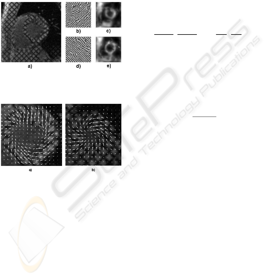
Figure 3: Given an incoming tagged frame a), two Gabor
filter banks are applied to it, leading to a couple of complex
images. The wraped version of their phase is shown in b)
and d), while their amplitudes in c) and e).
Figure 4: The resultant Harmonic Phase Flow over two an-
alyzed tagged frames, belonging to base a) and apex b).
Let {I
t
(x,y)}
T
t=0
denote a TMR sequence (fig.3 a))
and V
t
(x,y) the vector field matching frames at times
t and t + 1. The HPF estimation of such vector pro-
ceeds in two stages: extraction of a representation
space capturing local deformations and feature track-
ing within a variational framework.
The representation space is two dimensional (see
fig.3 b) and d)) and is obtained by assigning to each
point the maximum response of two Gabor filter
banks (one for each tag direction). The Gabor filters
are centered around the main frequency of tags and
tuned for each myocardial cut (base and apex). The
complex images in the representation space will be
noted by (I
t
1
,I
t
2
) and their phase and amplitude by Φ
k
and Λ
k
, respectively. On one hand, it can be shown
(Osman et al., 1999) that Φ
k
(fig.3 b) and d)) is a
material property of the tissue that remains constant
along the cardiac cycle. Since the brightness con-
stancy constrain is met, classical optical flow (Horn
and Schunck, 1981) can be applied two track both
phases. On the other hand, Λ
k
(fig.3 b) and d)) pro-
vides a measure of the reliability of the phase values
detected by the Gabor filter banks.
The variational framework we propose regularizes
the deformation field at areas where Λ
k
drops. The
searched vector field, V
t
(x,y) = (U
t
(x,y),V
t
(x,y)),
should minimize the energy:
Z
(1 − (α
1
+ α
2
)/2)
2
ε
2
reg
| {z }
+
Z
[α
2
1
ε
2
1
+ α
2
2
ε
2
2
]
| {z }
Regularity Matching
(1)
where the matching and the regularizing terms are de-
fined as:
ε
k
= Φ
kx
U + Φ
ky
V + Φ
kt
ε
reg
= k∇V k
2
= k∇Uk
2
+ k∇V k
2
for Φ
kx
, Φ
ky
, Φ
kt
, the partial derivatives of the k-essim
phase Φ
k
and the weighting functions α
k
’s given by
the amplitudes:
α
k
=
|Λ
k
|
max(|Λ
k
|)
The solution to the Euler Lagrange equations associ-
ated to the functional (1) is obtained by solving the
gradient descent scheme:
∂U
t
/∂t(x,y) =
−[(Φ
x
gΦ
x
)U
t
(x,y)+(Φ
x
gΦ
y
)V
t
(x,y) + Φ
x
gΦ
t
−(1 − α)
2
∆U
t
(x,y) + 2(1 − α)h∇α, ∇U
t
(x,y)i]
∂V
t
/∂t(x,y) =
−[(Φ
x
gΦ
y
)U
t
(x,y) + (Φ
y
gΦ
y
)V
t
(x,y) + Φ
y
gΦ
t
−(1 − α)
2
∆V
t
(x,y) + 2(1 − α)h∇α, ∇V
t
(x,y)i]
(2)
where h·,·i denotes the scalar product, ∇ and 4
stand for the gradient and Laplacian operators and
g = diag(α
2
1
,α
2
2
).
The solution to eq. (2) gives our Harmonic Phase
Flow. In (Garcia et al., 2006) we prove that it reaches
sub-pixel precision in experimental data. Two in-
stances, for basal and apical views, of its performance
are shown in figure 4.
3 NORMALIZED PARAMETRIC
DOMAIN
Comparing deformation fields from different se-
quences requires coping with inter and intra patient
A NORMALIZED PARAMETRIC DOMAIN FOR THE ANALYSIS OF THE LEFT VENTRICULAR FUNCTION
269

a)
b)
Figure 5: Comparison between image registration and map-
ping to normalized domain: registration a) and parametriza-
tion schemes b).
anatomical variability. In this Section we define a
parametrization that maps any left ventricle domain,
which we denote by LV , to a common normalized
domain, namely Ω = [0,1] × [0,1]. Such normalized
domain allows comparison of different vector fields
and, thus, computation of an average model of the LV
functionality. We note that LV parametrization is an
alternative to image registration (Zitova and Flusser,
2003), which maps image sequences to a reference
patient. The advantage of our approach is that, be-
sides giving an implicit registration, parametric coor-
dinates provide an intuitive way of moving on the my-
ocardial domain. Figure 5 sketches image registration
and LV parametrization. A registration scheme bases
on the mapping, Ψ
i j
, best matching two images I
i
and
I
j
(fig. 5.a). By using a parametrization, the left ven-
tricles, LV
i
and LV
j
, from different sequences, are
mapped to the common domain via Ψ
i
and Ψ
j
and the
composition Ψ
i
Ψ
−1
j
registers them (fig. 5.b).
The mapping from the image domain to the para-
metric domain is done by fitting a bi-dimensional B-
Spline over the target left ventricular region. B-Spline
fitting splits into fitting the initial spline at time 0 and
updating the initial shape under HPF deformation.
3.1 Initial Surface Fitting
The LV is a simple geometric entity since it is home-
omorphic (it identifies) to a torus. It follows that there
are two privileged directions, the circumferential (an-
gular) and the radial. If we parameterize these direc-
tions and normalize them in the range [0,1] we obtain
a universal (normalized) domain shared by all incom-
ing subjects. We define the initial parametrization,
Ψ
0
, of the undeformed left ventricular region, LV
0
,
in 3 stages. First we define a new coordinate system
based on anatomical landmarks in order to account
for affine differences among subjects. A B-spline
curve fitting of the inner (endocardium) and the outer
(epicardium) heart borders defines the angular coor-
dinate. Finally, the radial coordinate is obtained by
interpolating values between the two curves using a
bi-dimensional spline. The spline modelling accounts
for anatomical differences among subjects.
An affine coordinate system is defined by means
of an origin of coordinates, O, and two independent
axis, V
x
,V
y
. The new origin is defined as the center
of mass of a set of points segmenting the myocardial
borders (endocardium and epicardium). By the me-
chanics of rigid motion it follows that the new origin
compensates any translation. The new axis V
x
is a
unitary vector starting at O and pointing to the point,
P
as
, joining the right (RV) and left ventricles and sep-
arating the septum and the anterior walls. Finally the
vector V
y
is also unitary, orthogonal to V
x
and point-
ing oppositely to the septal wall. By considering the
anatomical key point P
as
as angular origin, we ac-
count for any rotational disparity among sequences.
Figure 6 describes the new reference system with the
key point P
as
highlighted with a solid black circle.
Figure 6: Affine reference accounting for affine transforma-
tions across sequences. The image coordinate system is at
the upper left corner and the coordinate system based on
anatomical features at the LV center.
Let (x
0
n
,y
0
n
) and (x
1
n
,y
1
n
) be, respectively, points on the
endocardium and epicardium in the new affine refer-
ence. Their angles, θ
0
n
and θ
1
n
, serve to fit a pair of
closed B-Spline curves, ψ
0
, ψ
1
, by minimizing:
ε
k
=
∑
N
k
n=1
kψ
k
(
θ
k
n
2π
) − (x
k
n
,y
k
n
)k
2
k = 0, 1
with
ψ
k
(u) =
∑
M
k
m=1
R
k
m
(u)P
k
m
k = 0, 1
for R
k
m
cubic blending functions and P
k
m
∈ R
2
control
points ensuring a closed curve (i.e. P
k
1
= P
k
M
k
−2
, P
k
2
=
P
k
M
k
−1
, P
k
3
= P
k
M
k
).
VISAPP 2008 - International Conference on Computer Vision Theory and Applications
270

In order to get the final parametrization we fit a
bi-dimensional spline to a uniform sampling of the
radial values (normalized in the range [0,1]) of the
two border splines at circumferential parameters u
i
=
(i−1)/(Nu−1). For each of them we obtain a couple
of points belonging to endocardium and epicardium
that are also uniformly sampled at radial values w
j
=
( j − 1)/(Nw − 1). This provides N
u
× N
w
myocardial
points, {X
0
i j
}
N
u
,N
w
i, j=1
, at the initial time. The parametric
map is obtained by fitting a bi-dimensional B-Spline
surface to such discrete set:
ε =
N
u
∑
i=1
N
w
∑
j=1
kΨ
0
(u
i
,w
j
) − X
0
i j
k
2
(3)
with
Ψ
0
(u,w) =
M
u
∑
n=1
M
w
∑
m=1
R
n
(u)S
m
(w)P
nm
In this case, R
n
are cubic blending functions, S
m
are
quadratic blending functions and P
nm j
∈ R
2
are con-
trol points ensuring a closed surface in the angular
direction.
3.2 General Surface Fitting
So far we have described the parametrization of the
initial left ventricular domain LV
0
. We next de-
scribe how to parameterize the deformed left ventric-
ular domain, LV
t
, at any stage of the systolic cycle
(t > 0). End systole is defined as the instant where
the area of the blood pool inside the LV is mini-
mum. This parametrization is also done by fitting a
B-Spline surface over the object of interest. The para-
metric domain Ω is uniformly sampled in a N
u
× N
v
grid defined by parameters u
i
= (i − 1)/(Nu − 1) and
w
j
= ( j −1)/(Nw − 1). These parameters are used to
obtain points in LV
0
(material points) by evaluating
Ψ
0
.
Myocardial points at positive times, X
t
i j
, are ob-
tained by iteratively applying the deformation maps,
V
t
, between two consecutive frames:
X
t
i j
=
½
X
0
i j
= Ψ
0
(u
i
,w
j
) t = 0
X
t
i j
= X
t−1
i j
+V
t−1
(X
t−1
i j
), t > 0
The mapping Ψ
t
is the minimum of a cost functional
of the form (3) given by changing X
0
i j
for X
t
i j
. Notice
that by keeping the same initial parameters, (u
i
,w
j
),
for the spatial points, the parametric domain Ω re-
mains the same for all times.
4 REGIONAL ANALYSIS OF THE
LV FUNCTION
In order to explore left ventricular dynamics, the vec-
torial data provided by HPF is mapped into the nor-
malized domain Ω. Unlike scalar data, that can be
directly mapped to Ω (via Ψ
t
), displacement vectors
are expressed in image coordinates. These global co-
ordinates depend on the acquisition conditions prone
to vary across patients. In order to get intrinsic coor-
dinates, vectorial data should be expressed in terms of
the local references associated to the LV parametriza-
tion. Instead of using the Jacobian of the inverse map,
we decompose (Spivak, 1999) vectors into their cir-
cumferential (corresponding to the u coordinate) and
radial (corresponding to the w coordinate) compo-
nents. The coordinates of the local parametric vectors
are given by the columns of the Jacobian of the map-
ping Ψ. We will note by
˜
V
t
= (
˜
U
t
,
˜
V
t
) the coordi-
nates of the deformation vectors in the local reference
system. In order to compare across patients they are
mapped back to the normalized domain:
UΩ
t
(u,v) :=
˜
U
t
(Ψ
t
(u,v))
V Ω
t
(u,v) :=
˜
V
t
(Ψ
t
(u,v))
The above vector fields allow a point-wise compar-
ison. In order to provide a more intuitive (for vi-
sual assessment) and robust (from the statistics point
of view) representation of the LV function, we ana-
lyze data within regions. Regions in Ω are defined by
giving a uniform grid. We will call grid cells along
the circumferential direction sectors and those along
the radial direction layers. A region division is de-
termined by the parameters defining the cells corners.
Thus, a division in N
sec
sectors and N
lay
layers is given
by {(u
i
,w
j
)}
N
sec
+1,N
lay
+1
i, j=1
, where u
i
= (i −1)/N
sec
and
w
j
= ( j − 1)/N
lay
. A given region, ω
IJ
, in sector I
and layer J is defined as:
ω
IJ
= {(u,w) ∈ Ω/ · · ·
u
I
≤ u ≤ u
I+1
,w
J
≤ w ≤ w
J+1
}
Regional values for the components of the displace-
ment fields are obtained as the mean of the com-
ponents inside each region ω
IJ
. We will denote by
V ω(I,J) = (Uω(I, J),V ω(I, J)) a regional vector in
sector I and layer J.
5 RESULTS
Our average model of the LV function has been ex-
tracted from a data set of 17 healthy volunteers, com-
posed by 12 males and 5 females aged between 23
A NORMALIZED PARAMETRIC DOMAIN FOR THE ANALYSIS OF THE LEFT VENTRICULAR FUNCTION
271

Figure 7: American Heart Association nomenclature for
myocardial segments. a) Basal and mid sectors: anterior
(a), anterolateral (al), inferolateral (il), inferior (i) infer-
oseptal (is) and anteroseptal (as). b) Apical sectors: anterior
(a), lateral (l), inferior (i) and septal (s).
and 55 (31±8.3). In order to avoid misalignments
due to breathing, sequences were recorded in breath-
hold. For the acquisition of the tagged sequences, a
Siemens Avanto 1.5 T (Erlangen, Germany) equip-
ment was used. Images have a resolution of 1.3 × 1.3
mm per pixel and a thickness of 6 mm per cut.
For each of the the 17 volunteers, we have consid-
ered apical (noted by A) and basal (noted by B) cuts.
Our regional model is composed of 3 layers, 15 sec-
tors and 9 equidistant stages of the systolic cycle. The
normality patterns are given by the average of the 17
regional values.
UN
t
l
(I, J) =
1
17
17
∑
n=1
Uω
t
l,n
(I, J)
V N
t
l
(I, J) =
1
17
17
∑
n=1
V ω
t
l,n
(I, J)
where I = {1,··· ,3}, J = {1, · · · , 15}, l = {B,A} and
t = {1,··· ,9} and they stand for layers, sectors, levels
and times, respectively.
The values obtained are showed in fig.8 for the
basal model and fig.9 for the apical one. In order to
provide a clearer and more intuitive model, functional
values are shown as arrows in a bull’s eye graphic di-
vided into 3 × 15 regions. For each model we show
the dynamical behavior in the 9 stages (given in per-
centages) of the systolic cycle. The arrows of each
region show the trend of the deformation, while the
color of the region codifies its magnitude (in pixels)
that is specified by the color bar shown in the right.
The bold line corresponds to the V
x
of our affine ref-
erence defined in Section 3.1. Although we have
considered a higher number of sectors, we will use
the nomenclature of the American Heart Association
(Cerqueira and et al., 2002) (depicted in figure 7) for
referencing them in the subsequent explanations.
From the graphics in fig.8, we can appreciate that
at basal levels the a and al sectors start to contract
while the rest present a counterclockwise rotation.
From 37.5% of the systole to the end, all sectors rotate
clockwise, though a, al and il sectors also experiment
some contraction. Concerning apical levels (fig.9), at
begin systole they experience a counterclockwise ro-
tation for all sectors but for the i. At 12.5% of the sys-
tolic cycle, the sectors s and i start to contract strongly
while the remaining continues rotating counterclock-
wise until 50%. From this stage on, sectors s and i
also present some clockwise rotation, while the re-
maining keep the same rotational tendency.
We have also explored whether the sectorial ten-
dency observed in the bull’s eye graphics is consis-
tent with the anatomical disposition of the ventricular
band segments (fig2). On a given ventricular band
segment, fiber orientation keeps approximately con-
stant (Torrent-Guasp et al., 2005). It follows that re-
gional motion should be similar on sectors belonging
to the same ventricular band segment. In order to ver-
ify such condition we have considered the regional
motion for the whole sequence described by the mo-
tion vectors for all times:
UN
l
(I, J) = (UN
1
l
(I, J),... , UN
9
l
(I, J))
V N
l
(I, J) = (V N
1
l
(I, J),... , V N
9
l
(I, J))
The set (UN
l
(I, J),V N
l
(I, J)) provides a feature
space for the regional motion of 18 dimensions. We
have performed a 2-class unsupervised clustering to
search for areas of uniform motion. We note that,
since the main motions of cardiac tissue are rotation
and contraction, the clusters detect contractile and ro-
tational areas.
The sequence regional motion clusters for base
and apex are given in fig.10.a and .b, respectively. On
top we have the colored segments of the bovine heart
and on bottom the classification of the bull’s eye re-
gions. The angular origin is depicted in all images in
solid bold line. The classification output is stamped
on the colored myocardium in double line ellipses.
Firstly we note that the regions of homogenous mo-
tion are consistent with the visual assessment of fig.8
and 9. Secondly, areas of uniform motion present a
good correlation with the division given by the ven-
tricular band segments. Mismatches (especially at
segment borders) are attributed to anatomical vari-
ability across species.
6 CONCLUSIONS AND FUTURE
WORK
In this paper we introduce a novel approach for ex-
ploring the regional dynamics of the left ventricle. We
VISAPP 2008 - International Conference on Computer Vision Theory and Applications
272
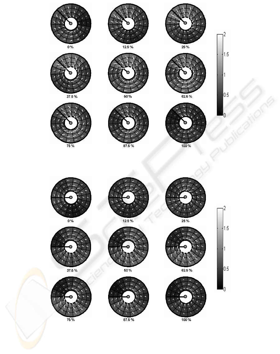
Figure 8: Regional Normality Patterns for Basal Level.
Figure 9: Regional Normality Patterns for Apical Level.
provide a general framework for computation of nor-
mality patterns and compute regional patterns from
healthy subjects. Our experiments prompt two rele-
vant issues. Firstly, motion is not uniform for a given
cut, so that, for a proper localization of the lesion, a
regional approach is more suitable than using global
scores (such as rotation or torsion (Garcia et al., 2006;
Lorenz et al., 2000)). Secondly, there is a strong rela-
tion between regional variability in heart motion and
the disposition of the ventricular band in space. The
promising results obtained for the 2D case encourage
extending the methodology to three dimensions.
A NORMALIZED PARAMETRIC DOMAIN FOR THE ANALYSIS OF THE LEFT VENTRICULAR FUNCTION
273

Figure 10: Correlation between ventricular band anatomy
(of a bovine heart) and uniform regional motion (of healthy
humans) for base a) and apex b).
ACKNOWLEDGEMENTS
We would like to thank Xavier Alomar from the Ra-
diology Department of the La Creu Blanca Clinic
for providing the tagged sequences. This work was
supported by the Spanish Government FIS projects
PI070454, PI071188 and FIS 04/2663. The last au-
thor is supported by The Ram
´
on y Cajal Program.
REFERENCES
Axel, L. and Dougherty, L. (1989). Mr imaging of motion
with spatial modulation of magnetization. Radiology,
171:841–845.
Cerqueira, M. and et al. (2002). Standardized myocar-
dial segmentation and nomenclature for tomographic
imaging of the heart. Circulation, 105:539–542.
Chandrashekara, R., Rao, A., Sanchez-Ortiz, G. I., Mohi-
addin, R. H., and Rueckert, D. (2003). Construction
of a statistical model for cardiac motion analysis using
nonrigid image registration. In Proc. IPMI.
Garcia, J., Gil, D., Barajas, J., Carreras, F., Pujades, S., and
Radeva, P. (2006). Characterization of ventricular tor-
sion in healthy subjects using gabor filters in a varia-
tional framework. In IEEE Proceeding Computers in
Cardiology.
Garot, J., Blumke, D., Osman, N., Rochitte, C., McVeigh,
E., and Zerhouni, E. (2000). Fast determination
of regional myocardial strain fields from tagged car-
diac images using harmonic phase mri. Circulation,
101(9):981–988.
Gotte, M., Germans, T., Russel, I., Zwanenburg, J., Marcus,
J., van Rossum, A., and van Veldhuisen, D. (2006).
Myocardial strain and torsion quantified by cardiovas-
cular magnetic resonance tissue tagging: Studies in
normal and impaired left ventricular function. J. A.
Coll. Cardiology, 48(10):2002–2011.
Guttman, M., Prince, J., and McVeigh, E. (1994). Tag
and contour detection in tagged mr images of the left
ventricle. Medical Imaging, IEEE Transactions on,
13(1):74–88.
Horn, B. and Schunck, B. (1981). Determining optical flow.
Artificial Intelligence, 17:185–204.
Jung, B., Kreher, B. W., Markl, M., and Henning, J. (2006).
Visualization of tissue velocity data from cardiac wall
motion measurements with myocardial fiber tracking:
principles and implications for cardiac fibers struc-
tures. European Journal of Cardio-Thoracic Surgery,
295:158–164.
Kocica, M., Corno, A., Carreras-Costa, F., Ballester-Rodes,
M., Moghbel, M., Cueva, C., Lackovic, V., Kanjuh,
V., and Torrent-Guasp, F. (2006). The helical ven-
tricular band: global, three-dimensional, functional
achitecture of the ventricular myocardium. European
Journal of Cardio-thoracic Surgery, 29:S21–S40.
Li, J. and Denney, T. (2006). Left ventricular motion re-
construction with a prolate spheroidal b-spline model.
Phys. Med. Biol., 51:517–537.
Lorenz, C., Pastorek, J., and Bundy, J. (2000). Delineation
of normal human left ventricular twist troughout sys-
tole by tagged cine magnetic resonance imaging. J
Cardiov. Magn. Reson., 2(2):97–108.
Luo, G. and Heng, P. (2005). Lv shape and motion: B-
spline-based deformable model and sequential motion
decomposition. IEEE T Inf. Technol. B., 9(3):430–
446.
Osman, N. F., Kerwin, W. S., McVeigh, E. R., and Prince,
J. L. (1999). Cardiac motion tracking using cine
harmonic phase (harp) magnetic resonance imaging.
Magnetic Resonance in Medicine, 42:1048–1060.
Rao, A., Sanchez-Ortiz, G., Chandrashekara, R., Lorenzo-
Valdes, M., Mohiaddin, R., and Rueckert, D. (2003).
Construction of a cardiac motion atlas from mr us-
ing non-rigid registration. In Functional Imaging and
Modeling of the Heart.
Spivak, M. (1999). A Comprehensive Introduction to Dif-
ferential Geometry, vol. 1 (3rd edition). Publish or
Perish, Inc.
Torrent-Guasp, F., Kocica, M., Corno, A., Komeda, M.,
Carreras-Costa, F., Flotats, A., Cosin-Aguilar, J., and
Wen, H. (2005). Towards a new understanding of
the heart structure and function. European Journal
of Cardio-thoracic Surgery, 27:191–201.
Waldman, L., Nosan, D., Villarreal, F., and Covell, J.
(1988). Relation between transmural deformation and
local myofiber direction in canine left ventricle. Circ.
Res., 63 (3):550–62.
Zerhouni, E., Parish, D., Rogers, W., Yang, A., and Shapiro,
E. (1988). Human heart: tagging with mr imaging–
a method for noninvasive assessment of myocardial
motion. Radiology, 169(1):59–63.
Zitova, B. and Flusser, J. (2003). Image registration meth-
ods: A survey. Im. Vis. Comp., 21:977–1000.
VISAPP 2008 - International Conference on Computer Vision Theory and Applications
274
