
IMAGE COMPLETION USING A DIFFUSION DRIVEN MEAN
CURVATURE FLOW IN A SUB-RIEMANNIAN SPACE
Gonzalo Sanguinetti
Instituto de Ingenier
´
ıa Electrica, Universidad de la Rep
´
ublica, Montevideo, Uruguay
Giovanna Citti
Dipartimento di Matematica, Universit
`
a di Bologna, Bologna, Italy
Alessandro Sarti
Dipartimento di Elettronica, Informatica e Sistemistica, Universit
`
a di Bologna, Bologna, Italy
Keywords:
Perceptual completion.
Abstract:
In this paper we present an implementation of a perceptual completion model performed in the three dimen-
sional space of position and orientation of level lines of an image. We show that the space is equipped with
a natural subriemannian metric. This model allows to perform disocclusion representing both the occluding
and occluded objects simultaneously in the space. The completion is accomplished by computing minimal
surfaces with respect to the non Euclidean metric of the space. The minimality is achieved via diffusion driven
mean curvature flow. Results are presented in a number of cognitive relevant cases.
1 INTRODUCTION
Perceptual completion is performed by the mam-
malian visual system in a number of phenomenologi-
cal cases, deeply studied by psychology of Gestalt to
understand the underlying structure of visual process-
ing in humans. The most common examples compre-
hend modal completion, amodal completion, trans-
parency, intersection and self intersection of curves
(Kanisza, 1979). Modal completion is the process of
filling the missing part of an object and building a per-
cept that is phenomenally undistinguishable from real
stimuli. It gives rise to the well known phenomenon
of illusory boundaries (or subjective contours) and it
takes place often to complete occluding objects (in
Fig. 1(a) the completed triangle is occluding the 3
circles). Amodal completion (Fig. 1(b)) is a percep-
tual modality for integrating missing parts of partially
occluded objects. Since the occluded figure underlies
the occluding one, it is completed without any senso-
rial counterpart. In case of transparency (Fig. 1(c))
and curve intersection (Fig. 1(d)), both occluding and
occluded figures are visible in the scene and the per-
ceptual system is able to disambiguate them and rec-
ognize them as different objects. A point made clear
by the studies of phenomenology of perception is that
in all cases of completion both the occluding and the
occluded objects are perceived at the same time in the
scene and therefore there are points in the input stim-
ulus corresponding to more than one figure at the per-
ceptual level. Many computer vision techniques have
been proposed to model perceptual completion. ei-
ther heuristically based or biologically inspired. Rec-
tilinear and curvilinear subjective contours have been
modeled by D.Mumford with Euler elastica as ex-
tremality points of curvature functionals (Nitzberg
and Mumford, 1990) and by stochastic fields as so-
lution of the Fokker-Planck equation (Williams and
Jacobs, 1995). In the latter case the stochastic com-
pletion field represents the likelihood that a comple-
tion joining two contour fragments passes through
any given position and orientation in the image. An
extension taking into account also the curvature has
been proposed in (August and Zucker, 2003). Amodal
completion has been accomplished by a number of
techniques. In (Masnou and Morel, 1998) (Ambro-
46
Sanguinetti G., Citti G. and Sarti A. (2008).
IMAGE COMPLETION USING A DIFFUSION DRIVEN MEAN CURVATURE FLOW IN A SUB-RIEMANNIAN SPACE.
In Proceedings of the Third International Conference on Computer Vision Theory and Applications, pages 46-53
DOI: 10.5220/0001075800460053
Copyright
c
SciTePress

(a) Modal completion (b) Amodal completion
(c) Transparency (d) Curve intersection
Figure 1: Examples of perceptual completion.
sio and Masnou, 2005) an extension of the Mumford
functional to level lines has been used to fill miss-
ing regions. Digital inpainting has been introduced
as a technique to diffuse existing information on the
boundary toward the interior region (Bertalm
´
ıo et al.,
2000) (Ballester et al., 2001). A total variation ap-
proach has been proposed in (Chan and Shen, 2001).
All these techniques consider the perceptual space in
which completion is performed has the same dimen-
sionality of the image. This could be a restriction
in case we are interested in the presence of recon-
structed occluding and occluded objects in the scene,
as in case of mammalian vision. To overcome this re-
striction, in (Citti and Sarti, 2006) has been proposed
a completion model based on the functional architec-
ture of the visual cortex, where completion is fully
performed in the rototranslation group R
2
× S
1
, al-
lowing the simultaneous reconstruction of occluding
and occluded objects. This model is an extension of
the one proposed in (Petitot and Tondut, 1999) where
curves are lifted in the three dimensional Heisenberg
group. Another higher dimensional model has been
introduced in (Ben-Shahar and Zucker, 2004) and in
(Medioni, 2000).
Following (Citti and Sarti, 2006), a two dimen-
sional image is lifted to a surface in the 3-dimensional
sub-Riemannian space, an occlusion is considered as
a hole in the surface, and the proposed model com-
plete the missing part of the image with a minimal
surface. Computing a minimal surface in the hole
and re-projecting it over the image domain, we find
the same level lines as Morel and Masnou have found
in (Masnou and Morel, 1998) minimizing an elastica
based functional.
In (Hladky and Pauls, 2005) the authors proposed
a very fast method for finding the minimal surface ex-
plicitly interpolating the level lines represented in the
Sub-Riemannian space even if it is not well suited for
simultaneous representation of occluded and occlud-
ing objects.
The main objective of this paper is to propose a
computational technique for finding minimal surfaces
by diffusion driven mean curvature flow. The tech-
nique is able to simultaneously construct occluded
and occluding objects. The surface is represented as a
thin concentrated mass, suitably diffused and concen-
trated with a two step algorithm adapted to the sub-
Riemannian metric. The diffusion driven method was
first introduced in the Euclidean settings in (Merriman
et al., 1998).
The paper is organized as follows:
• In section 2 we explain the lifting of the image to
the 3D position-orientation space and describe the
subriemannian structure of the space.
• In section 3 the main model of image completion
is proposed and discussed in detail.
• In section 4 we present the numerical scheme for
the equations presented in previous sections.
• In section 5 we describe the experiments realized
and provide the results obtained.
• Finally, conclusions are presented.
2 THEORETICAL BACKGROUND
2.1 Lifting of the Image Level Lines in a
3-Dimensional Space
An image I can be represented as a bounded func-
tion defined on a domain M ⊂ R
2
, I : M → R
+
. The
points of M have coordinates (x, y). At every point
of the image we detect the tangent direction to level
lines(I
y
,−I
x
), where I
x
and I
y
are the components of
the image gradient. If θ is the angle between the tan-
gent and the x-axis the tangent can be rewritten as
(cos(θ),sin(θ)).
We want to define the orientation independently of
the versus of the tangent vector. Therefore, we iden-
tify a tangent vector with its opposite one. This means
that angles which differ form π will be identified, and
θ(x,y) = −arctan(I
x
/I
y
) , θ ∈ S
1
,
IMAGE COMPLETION USING A DIFFUSION DRIVEN MEAN CURVATURE FLOWIN A SUB-RIEMANNIAN
SPACE
47
where S
1
is the set of angles [0,π].
To every point (x,y) is associated a three dimen-
sional vector (x,y,θ), in a new space homeomorphic
to R
2
×S
1
. Since the process is repeated at each point,
each level line is lifted to a new curve in the three
dimensional space. We will call admissible curve a
curve in R
2
× S
1
if it is the lifting of a level line.
2.2 The Tangent Bundle and the
Integral Curves
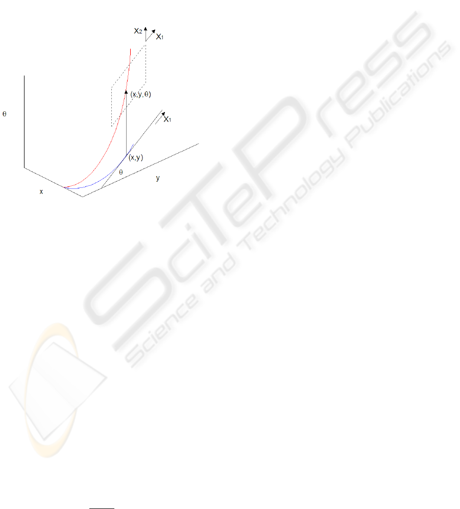
Figure 2: A lifted level line.
A tangent vector to the lifted curve has the same two
first components as the tangent vector to the level line,
i.e. a real multiple of (cos(θ),sin(θ)), and it has the
third component in the direction (0,0,1). Hence it
can be represented as a linear combination of the vec-
tors (cos(θ), sin(θ), 0) and (0,0,1) which, from now
on, will be called
~
X
1
and
~
X
2
respectively. The set of
vectors α
1
~
X
1
+α
2
~
X
2
defines a plane and every admis-
sible curve is tangent to a vector of the plane. Hence
an admissible curve satisfies the differential equation:
γ
0
(t) = α
1
~
X
1
(t)+ α
2
~
X
2
(t)
It is well known that the ratio α
2
/α
1
is the the curva-
ture k(t) of its 2D projection, the level line of I.
2.3 Curve Length’s and Metric of the
Space
If we equip the tangent planes with an Euclidean met-
ric then the length of an admissible curve can be com-
puted as usual integrating the tangent vector.
λ(γ)(t) =
Z
t
0
kγ
0
(s)kds =
Z
t
0
kα
1
~
X
1
+ α
2
~
X
2
kds
=
Z
t
0
α
1
p
1 + k
2
ds (1)
In order to define a distance in term of the length, we
need to answer the following question: Is it possible
to connect every couple of points of R
2
× S
1
using an
integral curve?
This is not a simple question taking into account
that in every point we have only directions which are
linear combinations of two vectors even if we are im-
mersed in a three dimensional space. However, the
answer is yes and it will become clear in the exam-
ple below. Otherwise, see (Citti and Sarti, 2006) for a
detailed justification.
Consequently, it is possible to define a notion
of distance between two points p
0
= (x
0
,y
0
,θ
0
) and
p
1
= (x
1
,y
1
,θ
1
):
d(p
0
, p
1
) = inf{λ(γ) : γ is an admmisible curve
connecting p
0
and p
1
} (2)
In the Euclidean case this infimum is realized by a
geodesic that is a segment. Here, the geodesics are lo-
cally curvilinear. The metric induced by (2) is clearly
Non-Euclidean, moreover it is not even Riemannian.
With the chosen metrics on the tangent plane, the
space co-metric is given by:
g =
cos(θ) 0
sin(θ) 0
0 1
cos(θ) sin(θ) 0
0 0 1
=
cos
2
(θ) cos(θ)sin(θ) 0
cos(θ)sin(θ) sin
2
(θ) 0
0 0 1
Since the matrix g is not invertible, it can not induce
a Riemannian metric on the space. Spaces equipped
with Sub-Riemannian metrics appears often when
one of the dimensions is a state variable depending
on the others. In this case the state variable is θ.
2.4 The Lifted Surface as an Implicit
Function
When every point of an entire image is lifted up, a
three dimensional surface is constructed as:
Σ =
(x,y,θ) ∈ R
2
× S
1
: θ(x, y) = − arctan(I
x
/I
y
)
We can identify the lifting of an image with the lifting
of every level line. This point of view allows us to
understand a remarkable property of the lifted surface.
In fact, since two level lines of an image never cross,
also the lifted level lines don’t do it. Then we say
that the lifted surface is foliated by the lifted curves
(see Fig. 3). We will call rule an admissible curve
foliating a surface.
VISAPP 2008 - International Conference on Computer Vision Theory and Applications
48
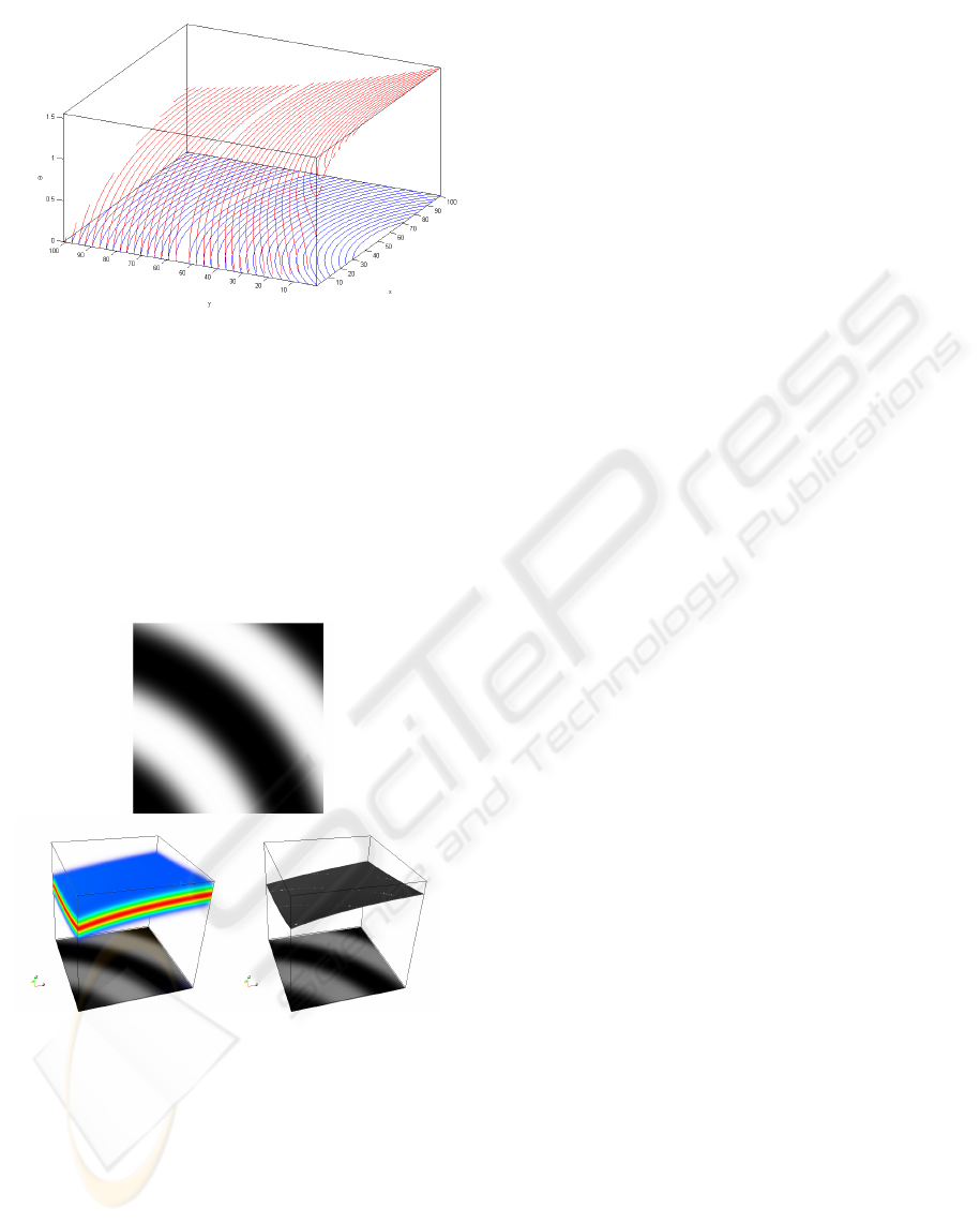
Figure 3: A lifted image is a surface foliated by the lifted
level lines.
Let’s now represent the surface in terms of the im-
plicit function
u(x,y,θ) = [cos (θ + arctan(I
x
/I
y
))]
2
(3)
For every coordinate (x,y) this function attains its
maximum in the variable θ in correspondence to a
point (x,y,
¯
θ) of the surface. The cosine function is
Figure 4: The lifted image can be viewed as a thick surface
and the surface obtained with eq. 4.
chosen in order to have periodicity of u in the third
coordinate since it is an angle. Note we have imposed
that the maximum value of u is 1.
The surface Σ can be represented as the zero level
set of the function u
θ
:
Σ = {(x,y,θ) ∈ R
2
× S
1
: ∂
θ
u(x,y,θ) = 0,
∂
θθ
u(x,y,θ) < 0} (4)
The condition over ∂
θθ
u is imposed in order to
avoid minima of u.
2.5 Sub-riemannian Differential
Operators
We will define differential operators acting over the
function u, in terms of the subriemannian structure
introduced before on the space R
2
×S
1
, instead of the
Euclidean one. We will need to define two differen-
tial operators X
1
and X
2
which play the role of the
Euclidean partial derivatives, and have the same coef-
ficients as the vector fields
~
X
1
and
~
X
2
. Hence
X
1
= cos(θ)∂
x
+ sin(θ)∂
y
, X
2
= ∂
θ
.
Accordingly we define the Sub-Riemannian gra-
dient as:
∇
SR
u = (X
1
u,X
2
u).
The notation SR (Sub-Riemannian) will be used in
order to avoid confusions with the classical operators.
We define the so called sub-laplacian operator, which
is the analogous of the classical laplacian in this struc-
ture:
∆
SR
u = X
2
1
u + X
2
2
u
= cos
2
(θ)u
xx
+ sin
2
(θ)u
yy
+
2cos(θ)sin(θ)u
xy
+ u
θθ
(5)
and we define the subriemannian diffusion equation
as:
u
t
= ∆
SR
u.
Despite of the fact the sublaplacian operator is built
just with two directional derivatives in a 3 dimen-
sional space, the diffusion process reaches every
point due to the connectivity property of the sub-
riemannian geometry.
2.6 Differential Geometry of the
Surface
Since the surface Σ, is the zero level set of the function
u
θ
= X
2
u, it is possible to define geometrical prop-
erties of Σ, in terms of the function u
θ
and its sub-
riemannian derivatives. The subriemannian gradient
∇
SR
u
θ
is orthogonal to the surface (w.r. of the subrie-
mannian metric), and an admissible tangent vector is
(−X
2
u
θ
,X
1
u
θ
). Correspondingly the rules on the sur-
face have the expression
γ
0
= −X
2
u
θ
~
X
1
+ X
1
u
θ
~
X
2
. (6)
Analogously the diffusion on the surface, which is
the diffusion along the rules, is expressed in terms of
∇
SR
u
θ
.
The foliation feature suggests a natural notion
of area in the sub-riemannian structure R
2
× S
1
.
Indeed the area of a lifted surface can be defined as
IMAGE COMPLETION USING A DIFFUSION DRIVEN MEAN CURVATURE FLOWIN A SUB-RIEMANNIAN
SPACE
49

the integral of the lengths of every rule. With this
definition, a minimal surface with assigned boundary
conditions is obtained requiring every rule to have
minimal length.
3 THE COMPLETION MODEL
3.1 Basic Model
In this section we present our completion model in the
rototraslation group, (see also (Citti and Sarti, 2006))
Let’s consider an image with an occlusion and let
us call D the missing part in the two dimensional do-
main. In order to complete it, we lift the image to a
surface in the Sub-Riemannian space. This lifted sur-
face will have a hole, which will be completed with a
minimal surface. Indeed, using relation (1), in (Citti
and Sarti, 2006) it has been proved that the subrie-
mannian minimization of the surface area gives rise to
the minimization on the rules on the surfaces, whose
projection are the elastica curves. Hence the mini-
mization of the first order area functional on R
2
× S
1
correspond to the minimisation of a second order cur-
vature functional on the image plane (Ambrosio and
Masnou, 2005) (Masnou and Morel, 1998).
The method we will use is the following: first we
lift the non occluded part of the image with eq. (3) to
a function u defined on (R
2
\D)× S
1
. In the occluded
region D × S
1
we assign value zero to the function u.
Later we built an initial surface in the missing region.
Finally we evolve this surface with an approximated
diffusion driven mean curvature flow until it becomes
minimal. This is a two step algorithm of diffusion and
concentration, as shown in (Citti and Sarti, 2006):
• Diffusion of existing information in the subrie-
mannian space with the sub-laplacian.
• Concentration of diffused information on the fiber
S
1
over every point (x, y).
3.2 Algorithmic Implementation
The image I is lifted to a surface, represented by the
maxima over the fiber S
1
of a function u, by using
equation (3) The first step is to propagate existing in-
formation from the boundary of the missing region
D × S
1
with sub-riemannian diffusion:
∂
t
u =
∆
SR
u if (x,y, θ) ∈ D × S
1
∂
θθ
u if (x,y,θ) ∈ (R
2
\ D) × S
1
,t ∈ [0,h]
u(0) = u
0
(7)
This first step is necessary to initialize the func-
tion u to be a rough solution, which will be refined by
diffusion driven mean curvature flow.
In fact after the initial propagation, a mean cur-
vature evolution of the function u is implemented by
using a two step iterative algorithm consisting in al-
ternative diffusion and concentration:
• Diffuse with the Sub-Laplacian operator (5) for a
short time with fixed boundary conditions in the
boundary of D × S
1
.
In the occluded region we diffuse using the sub-
Laplacian operator. This operator propagates data
in the direction of the vectors X
1
and X
2
. The dif-
fusion in the direction of X
1
alone would expand
into the occlusion the information taken from the
boundary just in a straight line parallel to the (x,y)
plane. By adding the diffusion in the X
2
direc-
tion, we allow propagation on curvilinear paths
on R
2
× S
1
, even if we make thicker the surface
represented by u as a side effect. Outside D × S
1
we use the equation u
t
= u
θθ
just to keep the same
thickness of the surface as in the interior of D×S
1
.
Note that if we just use this equation for a short
time the maximum of u is not moved and there-
fore the surface Σ does not change. For the dis-
occlution problem it is only necessary to consider
values of u near the boundary of D × S
1
. Only
this values will be propagated inside D ×S
1
. Nev-
ertheless, for improving the visualization we will
consider a larger domain outside D × S
1
.
• Concentrate the function u over the surface, i.e.
make thinner the thick version of the surface.
After diffusing u for a period of time h, we per-
form a concentration over its maximum and denote ¯u
the new function which implicitly define the concen-
trated surface:
¯u(x,y,θ) =
u(x,y,θ)
u
max
(x,y)
γ
, γ > 1 (8)
where:
u
max
(x,y) = max
θ∈S
1
{u(x,y,θ)} (9)
This procedure renormalize the function u in such a
way that the maximum over each fiber is 1. The con-
centration, obtained elevating the function u to a suit-
able power greater than one, preserves the value of the
maximum and reduces all the other values of u. Thus
this mechanism concentrates the function around its
maximum.
3.3 Multiple Concentration
The three dimensionality of the space allows the co-
existence of occluded and occluding objects at the
VISAPP 2008 - International Conference on Computer Vision Theory and Applications
50
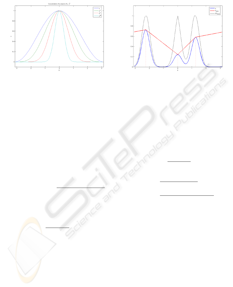
Figure 5: Concentration.
same time. In terms of the function u it means that
we expect to have more than one maximum in each
fiber. However, the equation described before (9), al-
lows only one maximum per fiber. The method de-
scribed above could be slightly modified in order to
avoid this limitation. In particular we propose the fol-
lowing renormalization criterion.
We first detect the maxima on a fiber over the point
(x,y) as the set {θ ∈ S
1
,∂
θ
u(x,y,θ) = 0, ∂
θθ
u(x,y,θ) <
0}. We call them θ
1
,...,θ
n
with θ
i
< θ
i+1
. Then we
construct a piecewise linear function u
norm
(Fig. 6 )
connecting every local maximum detected and peri-
odic in the variable θ:
u
norm
(x,y,θ) = u(x, y,θ
j
) + (10)
(θ − θ
j
)
u(x,y,θ
j+1
) − u(x, y,θ
j
)
θ
j+1
− θ
j
with θ ∈ [θ
j
,θ
j+1
].
We use eq (10) to re-normalize every single col-
umn of u as follows:
¯u(x,y,θ) =
u(x,y,θ)
u
norm
(x,y,θ)
γ
, γ > 1
After renormalization the function ¯u keep the same
points of maximum as the function u and attains value
1 at each of these points.
As we mentioned before, this modification allows
more than one maximum on each fiber. Hence
applying iteratively this improved concentration
technique and the sub-riemannian diffusion, we
compute minimal surfaces, in R
2
× S
1
which are
union of graphs of the variable (x, y), which can
partially overlap. It corresponds to the completion of
both occluding and occluded object.
Figure 6: Improved re-normalization.
4 NUMERICAL SCHEME
For the diffusion we use a finite difference scheme.
Let us consider a rectangular grid in space-time
(x,y,θ,t). The grid consist of a set of points
(x
l
,y
m
,θ
q
,t
n
) = (l∆x,m∆y, q∆θ, n∆t).
Following the standard notation, we denote by
u
n
lmq
the value of the function u at a grid point. We
use forward differences in order to approximate the
time derivative:
D
t
u =
u
n+1
lmq
− u
n
lmq
∆t
and center differences for the spatial ones:
D
x
u
n
lmq
=
u
n
(l+1)mq
− u
n
(l−1)mq
2∆x
D
xx
u
n
lmq
=
u
n
(l+1)mq
− 2u
n
lmq
+ u
n
(l−1)mq
(∆x)
2
The second directional derivatives are approximated
with:
D
11
u
n
lmq
= cos(θ
q
)
2
D
xx
u
n
lmq
+ sin(θ
q
)
2
D
yy
u
n
lmq
+2cos(θ
q
)sin(θ
q
)D
xy
u
n
lmq
D
22
u
n
lmq
= D
θθ
u
n
lmq
We impose Neumann boundary conditions on x and
y and periodic boundary conditions on the third di-
rection θ. The time step ∆t is upper bounded by the
usual Courant-Friedrich-Levy condition that ensures
the stability of the evolution [11].
5 EXPERIMENTS AND RESULTS
5.1 Macula Cieca
In this experiment we consider the completion of a
figure that has been partially occluded. This example
IMAGE COMPLETION USING A DIFFUSION DRIVEN MEAN CURVATURE FLOWIN A SUB-RIEMANNIAN
SPACE
51
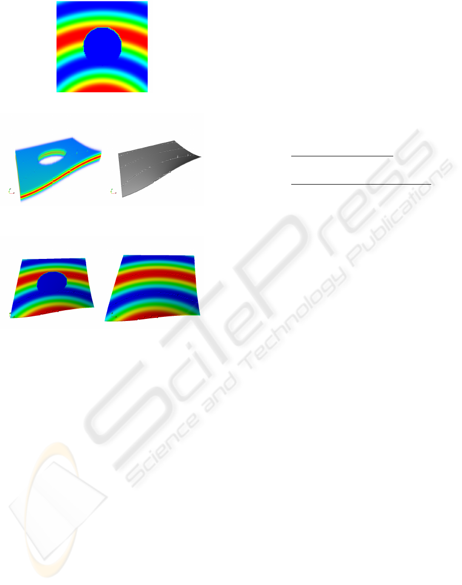
(a) Original Image.
(b) Initially lifted surface and the minimal surface com-
puted.
(c) Gray level diffusion.
Figure 7: Macula cieca example.
mimics the missing information due to the presence
of the macula cieca (blind spot) that is modally com-
pleted by the human visual system. As described in
the previous section the occluded image is lifted to a
surface with a hole in the three dimensional space and
an initial surface is defined in the missing part with a
classical Euclidean diffusion equation. Then the sur-
face is evolved applying iteratively equations (7) and
(9) until a steady state is achieved.
The image dimensions are 100 × 100 pixels, and
we use 100 values to discretize the variable θ. For
the preprocessing step 100 iterations of the Euclidean
heat equation were made using a time step of ∆t = 0.1.
The steady state was reached after 20 iterations with a
concentration power in (8) of γ = 2 and 20 steps with
∆t = 0.1 of the subriemannian heat equation (7).
At this point we have completed the missing in-
formation of the lifted surface with a minimal surface
in the Sub-Riemannian space. The lifting and com-
pletion processes take into account just the direction
of the level lines of the image, as a geometric infor-
mation. Then the intensity information of the image
is completely missed.
Let’s define a function v extending the values of
the image I on the 3 dimensional space, and constant
in the variable θ:
v(x,y,θ) =
I(x,y) (x,y,θ) ∈ (R
2
\D) × S
1
0 (x,y,θ) ∈ D × S
1
We will use a Laplace Beltrami diffusion algorithm in
the sub-riemannian setting to propagate the function v
along the rules of the minimal surface. Since the rules
of the surface, defined in (6) only depend on ∇
SR
u
θ
,
the Laplace Beltrami operator is a linear operator in
the variable v whose coefficients depend on ∇
SR
u
θ
:
v
t
=
|X
2
u
θ
|
2
X
2
1
v + |X
1
u
θ
|
2
X
2
2
v
X
2
1
u
θ
+ X
2
2
u
θ
−
X
1
u
θ
X
2
u
θ
X
1
X
2
v − X
1
u
θ
X
2
u
θ
X
2
X
1
v
X
2
1
u
θ
+ X
2
2
u
θ
5.2 Occlusion
In Figure 8 an occlusion problem is considered. The
initial image (top) shows an underlying object par-
tially occluded by a vertical stripe. The human vi-
sual system simultaneously segments the occluding
object and amodally completes the occluded one, tak-
ing both at the same time as perceived units. In the
numerical experiment first the image is lifted in the
sub-riemannian space and the missing information is
completed. The result shows that the partially oc-
cluded object has been completed and the occluding
one has been segmented. Both objects are present at
the same time in the three dimensional space.
For this example the dimensions were again 100×
100 × 100 pixels. Non preprocessing step is needed.
The steady state was reached after 10 iterations with
a concentration power of γ = 2 in equation 8 and 10
steps with ∆t = 0.1 of the subriemannian diffusion
step.
6 CONCLUSIONS
In this paper we utilized a model of perceptual com-
pletion inspired from the visual cortex to perform
completion of occluding and occluded objects in im-
ages. In particular we achieved the task by computing
minimal surfaces in sub-riemannian space via diffu-
sion driven mean curvature flow. The implementation
has been performed with a two steps iterative algo-
rithm of diffusion and concentration. A new concen-
tration technique allowing more than one maximum
over the fibers has been proposed. This allows to com-
pute a set of graphs partially overlapped representing
the occluding and the occluded objects. Computa-
tional results on cognitive images have been achieved.
VISAPP 2008 - International Conference on Computer Vision Theory and Applications
52
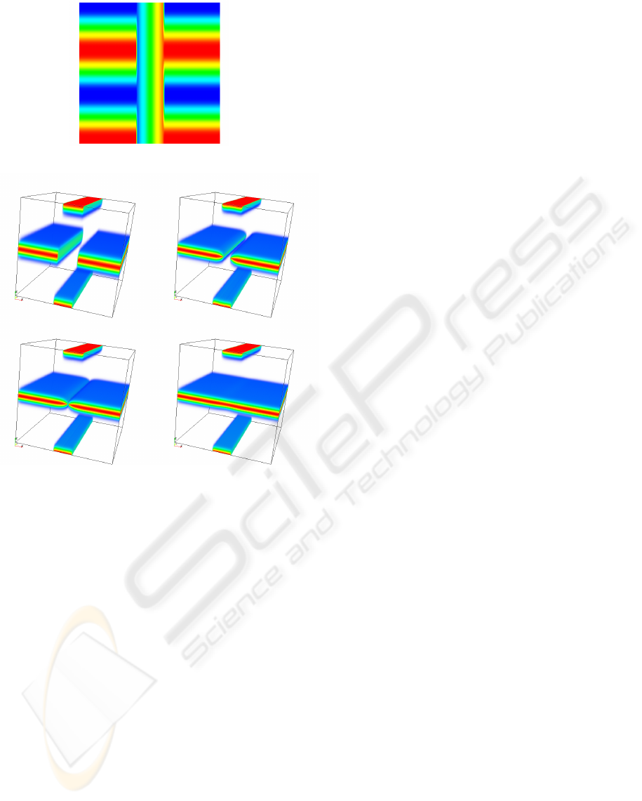
(a) Original Image.
(b) Some steps of the evolution.
Figure 8: Occlusion example: Mean Curvature Evolution
with 2 simultaneous surfaces.
ACKNOWLEDGEMENTS
This work was partially supported by ALFA
project II-0366-FA and NEST project GALA (Sub-
Riemannian geometric analysis in Lie groups) num-
ber 028766.
REFERENCES
Ambrosio, L. and Masnou, S. (2005). On a variational prob-
lem arising in image reconstruction.
August, J. and Zucker, S. W. (2003). Sketches with cur-
vature: The curve indicator random field and markov
processes. IEEE Trans. Pattern Anal. Mach. Intell,
25(4):387–400.
Ballester, C., Bertalm
´
ıo, M., Caselles, V., Sapiro, G., and
Verdera, J. (2001). Filling-in by joint interpolation of
vector fields and gray levels. IEEE Transactions on
Image Processing, 10(8):1200–1211.
Ben-Shahar, O. and Zucker, S. W. (2004). Geometri-
cal computations explain projection patterns of long-
range horizontal connections in visual cortex. Neural
Computation, 16(3):445–476.
Bertalm
´
ıo, M., Sapiro, G., Caselles, V., and Ballester, C.
(2000). Image inpainting. In SIGGRAPH, pages 417–
424.
Chan, T. F. and Shen, J. (2001). Mathematical models
for local nontexture inpaintings. Journal of Applied
Mathematics, 62(3):1019–1043.
Citti, G. and Sarti, A. (2006). A cortical based model of per-
ceptual completion in the roto-translation space. Jour-
nal of Mathematical Imaging and Vision, 24(3):307–
326.
Hladky, R. K. and Pauls, S. D. (2005). Minimal surfaces
in the roto-translation group with applications to a
neuro-biological image completion model. Comment:
35 pages, 15 figures.
Kanisza, G. (1979). Organization in Vision: Essays on
Gestalt Perception. Praeger, New York, NY.
Masnou, S. and Morel, J.-M. (1998). Level lines based dis-
occlusion. In ICIP (3), pages 259–263.
Medioni, G. (2000). Tensor voting: Theory and applica-
tions.
Merriman, B., Bence, J. K., and Osher, S. J. (1998). Diffu-
sion generated motion by mean curvature. Computa-
tional Crystal Growers Workshop, J. Taylor Sel. Tay-
lor (Ed).
Nitzberg, M. and Mumford, D. (1990). The 2.1-D sketch. In
International Conference on Computer Vision, pages
138–144.
Petitot, J. and Tondut, Y. (1999). Vers une neurog
´
eom
´
etrie.
fibrations corticales, structures de contact et contours
subjectifs modaux.
Williams, L. R. and Jacobs, D. W. (1995). Stochastic com-
pletion fields: A neural model of illusory contour
shape and salience. In ICCV, pages 408–415.
IMAGE COMPLETION USING A DIFFUSION DRIVEN MEAN CURVATURE FLOWIN A SUB-RIEMANNIAN
SPACE
53
