
AN AUTOMATIC WELDING DEFECTS CLASSIFIER SYSTEM
Juan Zapata, Ram´on Ruiz
Departamento de Electr´onica y Tecnolog´ıa de Computadoras,
Universidad Polit´ecnica de Cartagena,
Antiguo Cuartel de Antigones. Plaza del Hospital 1, 30202 Cartagena, Spain
Rafael Vilar
Departmento de Estructuras y Construcci´on,
Universidad Polit´ecnica de Cartagena,
Antiguo Hospital de Marina, Muralla del Mar s/n, 30202 Cartagena, Spain
Keywords:
Weld defect, connected components, principal component analysis, artificial neuronal network.
Abstract:
Radiographic inspection is a well-established testing method to detect weld defects. However, interpretation
of radiographic films is a difficult task. The reliability of such interpretation and the expense of training
suitable experts have allowed that the efforts being made towards automation in this field. In this paper, we
describe an automatic detection system to recognise welding defects in radiographic images. In a first stage,
image processing techniques, including noise reduction, contrast enhancement, thresholding and labelling,
were implemented to help in the recognition of weld regions and the detection of weld defects. In a second
stage, a set of geometrical features which characterise the defect shape and orientation was proposed and
extracted between defect candidates. In a third stage, an artificial neural network for weld defect classification
was used under three regularisation process with different architectures. For the input layer, the principal
component analysis technique was used in order to reduce the number of feature variables; and, for the hidden
layer, a different number of neurons was used in the aim to give better performance for defect classification
in both cases. The proposed classification consists in detecting the four main types of weld defects met in
practice plus the non-defect type.
1 INTRODUCTION
In the last five decades, Non Destructive Testing
(NDT) methods have gone from being a simple lab-
oratory curiosity to an essential tool in industry. With
the considerable increase in competition among in-
dustries, the quality control of equipment and mate-
rials has become a basic requisite to remain competi-
tive in national and international markets. Although it
is one of the oldest techniques of non-destructive in-
spection, radiography is still accepted as essential for
the control of welded joints in many industries such
as the nuclear, naval, chemical, aeronautical. It is
particularly important for critical applications where
weld failure can be catastrophic, such as in pressure
vessels, load-bearing structural members, and power
plants (Edward, 1993).
For the correct interpretation of the representa-
tive mark of a heterogeneity, a knowledge of welded
joint features and of the potential heterogeneities and
types of defect which can be detected using radio-
graphic welded joint inspection is necessary. Limi-
tations to correlating the heterogeneity and the defect
are imposed by the nature of the defect (discontinu-
ities and impurities), morphology (spherical, cylin-
drical or plain shape), position (superficial or internal
location), orientation and size. Therefore, the radio-
graphic welded joint interpretation is a complex prob-
lem requiring expert knowledge.
2 EXPERIMENTAL METHOD
Figure 1 shows the major stages of our welding de-
fect detection system. Digital image processing tech-
niques are employed to lessen the noise effects and
to improve the contrast, so that the principal ob-
jects in the image become more apparent than the
background. Threshold selection methods, labelled
techniques and feature extraction are used to obtain
260
Zapata J., Ruiz R. and Vilar R. (2008).
AN AUTOMATIC WELDING DEFECTS CLASSIFIER SYSTEM.
In Proceedings of the Third International Conference on Computer Vision Theory and Applications, pages 260-263
DOI: 10.5220/0001075902600263
Copyright
c
SciTePress
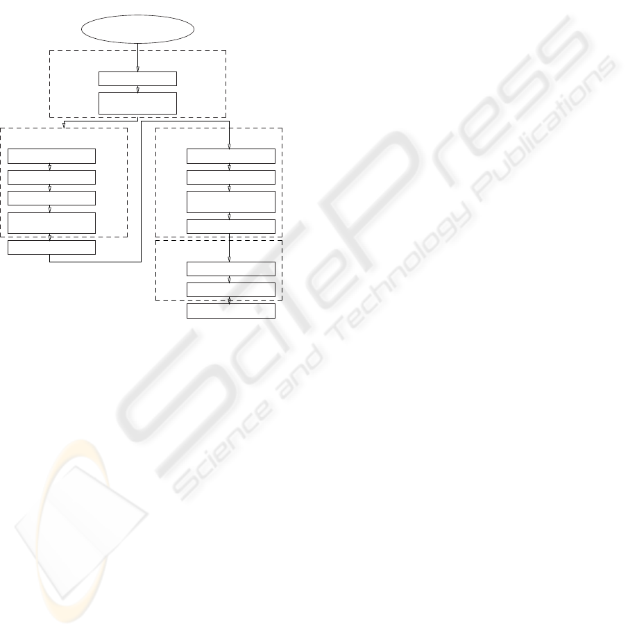
a feature discriminatory that can facilitate both the
weld region and defects segmentation. Finally, fea-
tures obtained are input pattern to artificial neural net-
work (ANN). Previously, principal component anal-
ysis (PCA) is first used to perform simultaneously
a dimensional reduction and redundancy elimination.
Secondly, an ANN is employed for the welding fault
identification task where three regularisation process
are employed in order to obtain a better generalisa-
tion.
Noise reduction
Contrast
enhacement
Preprocessing
Weld segmentation
Labelling
Weld region
Feature extraction
segmentation
ROI
Defect segmentation
Labelling
Defect
segmentation
Feature extraction
ANN
PCA
Regularization
Radiographic Image
Results
Thresholding Otsu Thresholding Otsu
Figure 1: Procedure for the automatic welding defect detec-
tion system.
After digitising the films (Zscherpel, 2000;
Zscherpel, 2002), it is common practice to adopt a
preprocessing stage for the images with the specific
purpose of reducing/eliminating noise and improving
contrast. Two preprocessing steps were carried out
in this work: in the first step, for reducing/eliminating
noise an adaptiveWiener filter (Lim, 1990) and Gaus-
sian low-pass filter were applied, while for adjusting
the image intensity values to a specified range to con-
trast stretch, contrast enhancement was applied in the
second step.
The last stage is the feature extraction in terms of
individual and overall charcateristics of the hetereo-
geneities. The output of this stage is a description of
each defect candidate in the image. This represents a
great reduction in image information from the origi-
nal input image and ensures that the subsequent clas-
sification of defect type and cataloguing of the degree
of acceptance are efficient. In the present work, fea-
tures describing the shape, size, location and intensity
information of defect candidates were extracted.
The dimension of the input feature vector of defect
candidates is large, but the components of the vectors
can be highly correlated and redundant. It is useful in
this situation to reduce the dimension of the input fea-
ture vectors. An effective procedure for performing
this operation is principal component analysis. This
technique has three effects: it orthogonalises the com-
ponents of the input vectors (so that they are uncorre-
lated with each other), it orders the resulting orthogo-
nal components (principal components) so that those
with the largest variation come first, and it eliminates
those components that contribute the least to the vari-
ation in the data set.
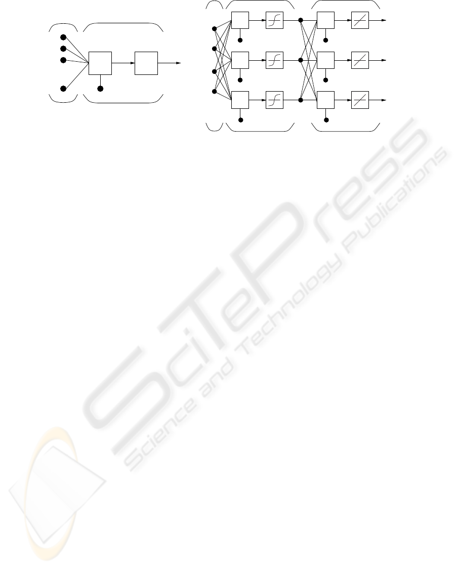
3 MULTI-LAYER
FEED-FORWARD ANN
A multiply-input neuron model is shown on the left
in Figure 2. The topology of the network used in this
work is illustrated on the right in Figure 2. Nonlin-
ear pattern classifiers were implemented using ANNs
of the supervised type using the error backpropaga-
tion algorithm and two layers, one hidden layer (S
1
neurons) using hyperbolic tangent sigmoid transfer
function and one output layer(S
2
= 5 neurons) using
a linear transfer function. In this work, a BFGS algo-
rithm (Dennis and Schnabel, 1983) was used to train
the network. The algorithm requires more computa-
tion in each iteration and more storage than the con-
jugate gradient methods, although it generally con-
verges in fewer iterations. The approximate Hessian
must be stored, and its dimension is n × n, where n
is equal to the number of weights and biases in the
network, therefore for smaller networks can be an ef-
ficient training function.
One of the problems that occur during neural net-
work training is called overfitting. The error on the
training set is driven to a very small value, but when
new data is presented to the network the error is large.
The network has memorised the training examples,
but it has not learned to generalise to new situations.
In this work, three methods was used in order to im-
prove generalisation. The first method for improving
generalisation is called regularisation with modified
performance function. This involves modifying the
performance function, which is normally chosen to
be the sum of squares of the network errors on the
training set. The second method automatically sets
the regularisation parameters. It is desirable to deter-
mine the optimal regularisation parameters in an au-
tomated fashion. One approach to this process is the
Bayesian regularisation (MacKay, 1992) (Foresee and
Hagan, 1997). The third method for improving gener-
AN AUTOMATIC WELDING DEFECTS CLASSIFIER SYSTEM
261
.
.
.
.
.
.
.
.
.
.
.
.
.
.
.
1
w
1,1
w
1,R
b
n a
Input
p
1
f
∑
p
1
p
2
p
2
p
3
p
3
p
R
.
.
.
p
R
Input
General neuron
∑
∑
∑
1
1
1
∑
∑
∑
1
1
1
w
1
1,1
w
1
S
1
,R
b
1
1
b
1
2
w
2
S
2
,S
1
w
2
1,1
b
2
1
b
2
2
Hidden layer Output layer
a
2
S
2
n
2
S
2
a
1
S
1
n
1
S
1
b
2
S
2
n
1
2
n
1
1
a
1
1
a
1
2
n
2
1
n
2
2
a
2
2
a
2
1
b
1
S
1
a = f(W p+ b)
a
2
= f
2
(W
2
f
1
(W
1
p+ b
1
) + b
2
)
Figure 2: Neuron model and network architecture.
alisation is called early stopping or bootstrap. In this
technique the available data is divided into three sub-
sets. The first subset is the training set, which is used
for computing the gradient and updating the network
weights and biases, in our case 50 % of data. The
second subset is the validation set, 25 % of data. The
third subset, 25 % of data, is the test set is not used
during the training process.
4 RESULTS AND CONCLUSIONS
To validate the proposed technique for the automatic
detection of weld defects, the same set of 86 radio-
graph images from the reference collection of the
IIW/IIS were used. In order to evaluate the perfor-
mance of the system, it is important to know if the
system is able to detect all defects. In this stage, our
system is able to obtain a sensibility of 100%, i.e. the
system detects as defect candidate all the defects ob-
served by the human expert. For a defect detection
system it is very important to have minimal loss in de-
fect regions even at the cost of increasing the number
of non-defectareas. The performanceis obtained with
a regression analysis between the network response
and the correspondingtargets. An artificial neural net-
work can be more efficient if varying the number of
neurons R in the input layer (by means of principal
component analysis) and S
1
in the hidden layer and
observing the performance of the classifier for each
defect and for each method of regularisation was pos-
sible to obtain the most adequate number of neurons
for the input and hidden layer and more appropriate
method of regularisation.
Figure 3 illustrates the graphical output of corre-
lation coefficient provided for the regression analysis
for each method of regularisation, i.e. using a mod-
ified performance function, Bayesian regularisation
and stopping early, in average for all classes. In gen-
eral, all outputs seem to track the targets reasonably
very well and all correlation coefficients are round-
ing 0.8. In some particular case, transversal crack
with Bayesian regularisation and stopping early meth-
ods for some determined number of PCA variation
and hidden layer neurons, the correlation coefficient
is not so good. These results are shown in Table 1 for
each one of the categories of regularisation and defect
types for a better interpretation. Underlined results
are the optimum values for our aim.
REFERENCES
Dennis, J. and Schnabel, R. (1983). Numerical Methods
for Unconstrained Optimization and Nonlinear Equa-
tions. Prentice-Hall.
Edward, G. (1993). Inspection of welded joints. In ASM
Handbook Welding, Brazing and Soldering, volume 6,
pages 1081–1088, Materials Park, Ohio. ASM Inter-
national.
Foresee, F. and Hagan, M. (1997). Gauss-newton approx-
imation to bayesian regularization. In Proceedings
of the 1997 International Joint Conference on Neural
Networks, pages 1930?–1935.
Lim, J. (1990). Two-Dimensional Signal and Image Pro-
cessing, pages 536–540. Prentice Hall, Englewood
Cliffs, NJ,.
MacKay, D. (1992). Bayesian interpolation. Neural Com-
putation, 4(3):415–447.
Zscherpel, U. (2000). Film digitisation systems for dir:
Standars, requirements, archiving and priting. 5 (05),
NDT.net (http://www.ndt.net).
Zscherpel, U. (2002). A new computer based concep for
digital radiographic reference images. 7(12), NDT.net
(http://www.ndt.net).
VISAPP 2008 - International Conference on Computer Vision Theory and Applications
262
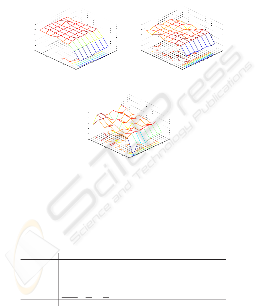
PCA variation Hidden layer neurons
Correlation Coeff.
MEAN FOR ALL DEFECT
Modified Performance Function
10
12
14
16
18
20
22
24
80%
90%
95%
99%
99.5%
99.9%
99.95%
99.99%
0
0.2
0.4
0.6
0.8
1
PCA variation Hidden layer neurons
Correlation Coeff.
MEAN FOR ALL DEFECT
Bayesian Regularization
10
12
14
16
18
20
22
24
80%
90%
95%
99%
99.5%
99.9%
99.95%
99.99%
0
0.2
0.4
0.6
0.8
1
PCA variation
Hidden layer neurons
Correlation Coeff.
MEAN FOR ALL DEFECT
Stop Early
10
12
14
16
18
20
22
24
80%
90%
95%
99%
99.5%
99.9%
99.95%
99.99%
0
0.2
0.4
0.6
0.8
1
Figure 3: Mean Correlation coefficient for each regularisation method.
Table 1: Better results for correlation coefficients (C.C.) for a specific number of neurons in the input layer (I. n.) and hidden
layer (H. n.) for each defect class and for each regularisation method.
Regularisation Method
Mod. perf. func. Bayes. regress. Stop. early
D
e
f.
No defect 0.9209 10 20 0.9042 7 22 0.9209 11 14
slag Incl. 0.7055 7 24 0.7209 11 10 0.7013 11 16
Poros. 0.7562 10 18 0.7204 7 20 0.7754 11 16
T. Crack 0.7978 11 22 0.8637 7 14 0.8637 11 12
L. Crack 0.9623 2 22 0.9623 8 20 0.9233 8 10
Mean 0.8041 11 20 0.7619 8 20 0.7802 11 12
C.C. I. n. H. n. C.C I. n. H. n. C.C. I. n H. n.
AN AUTOMATIC WELDING DEFECTS CLASSIFIER SYSTEM
263
