
ANISOTROPIC DIFFUSION BY QUADRATIC REGULARIZATION
Marcus Hund and B
¨
arbel Mertsching
University of Paderborn, Faculty of Computer Science
Electrical Engineering and Mathematics, GET Lab, Germany
Keywords:
Edge Preserving Smoothing, Noise Removal, Anisotropic Diffusion, Regularization.
Abstract:
Based on a regularization formulation of the problem, we present a novel approach to anisotropic diffusion
that brings up a clear and easy-to-implement theory containing a problem formulation with existence and
uniqueness of the solution. Unlike many iterative applications, we present a clear condition for the step size
ensuring the convergence of the algorithm. The capability of our approach is demonstrated on a variety of well
known test images.
1 INTRODUCTION
The idea of anisotropic diffusion in image process-
ing, i. e. diffusion along a preferred orientation, was
first introduced by Perona and Malik (Perona and Ma-
lik, 1990). Their method was designed to realize im-
age smoothing with simultaneous edge enhancement.
In this context an important issue is the relation of
the method to the scale space theory as introduced by
Witkin. In the last decade, the most important contri-
bution to the topic is the work of Weickert ((Weick-
ert, 1996), (Weickert, 1999)). Like Perona and Malik,
Weickert uses the diffusion equation
∂u
∂t
= ∇ · (D∇u) (1)
and provides a well-founded mathematical framework
(Weickert, 1996). He derives the diffusion tensor D
from a structure tensor description of the input image
in order to describe the local image structure. A ma-
jor drawback of the structure tensor description, espe-
cially combined with a Gaussian regularization, is the
high orientation uncertainty in the presence of junc-
tions in the image.
Even though there is a close relationship between
diffusion filters in the sense of eq. (1) and regu-
larization methods, one main difference is the fact
that the scale space in eq. (1) is given by the time
step t, i. e. the process converges to an one val-
ued image representing the maximum smoothed ver-
sion of the input image. Contrary to this the scale
space in regularization-based approaches is given by
a smoothing weight within an energy or cost func-
tional that has to be minimized. Although there ex-
ist a wide range of regularization-based approaches to
image processing (see e. g. (Ito and Kunisch, 1999),
(Nordstrom, 1989), (Aubert et al., 1997) and refer-
ences therein), we are not aware of a regularization-
based approach to anisotropic diffusion that brings
up a clear and easy-to-implement theory containing
a problem formulation with existence and uniqueness
of the solution and an iterative scheme with a scale
dependent step size that guarantees the convergence
of the method. Exactly this is what we present in
the following sections. In (Aubert et al., 1997) the
superiority of so called edge preserving models over
quadratic regularization is stated. Contrary to this, we
will show that edge preserving diffusion indeed can
be formulated as quadratic regularization.
The most suggesting application of edge preserving
regularization is image denoising. In (Portilla et al.,
2003) a good overview to existing denoising methods
is given. In an extensive quantitative evaluation Por-
tilla et al. show that their approach appears to be the
most accurate one compared to other state-of-the-art
methods. Therefore we will give a short comparison
to their method.
2 GLOBAL OPTIMIZATION
2.1 Problem Formulation
In our approach the discrete image is regarded as a
vector ξ
0
∈ R
(m·d)
with m being the total number of
101
Hund M. and Mertsching B. (2008).
ANISOTROPIC DIFFUSION BY QUADRATIC REGULARIZATION.
In Proceedings of the Third International Conference on Computer Vision Theory and Applications, pages 101-107
Copyright
c
SciTePress

pixels in the image and d the number of colors used.
Two assumptions are made about the cost function.
First, it should cause costs if the image elements ξ
(x,k)
differ from the initial pixel values ξ
(x,k)
0
. Second,
neighboring elements must satisfy a continuity con-
straint. This leads to a cost function of the form
P(ξ) =
1
2
·
d
∑
k=1
m
∑
i=1
(ξ
(i,k)
− ξ
(i,k)
0
)
2
+
c
4
·
d
∑
k=1
m
∑
i=1
∑
j∈U
i
w
i j
(ξ
(i,k)
− ξ
( j,k)
)
2
(2)
with ξ = (ξ
(1,1)
,...,ξ
(m,1)
,ξ
(1,2)
,...,ξ
(m,d)
)
T
with a
smoothness or scaling factor c. Here, U
x
is the neigh-
borhood of a given pixel x with a weighting factor
w
xi
> 0 with
∑
i∈U
x
w
xi
≤ Q :=
∑
i∈U
x
1. Note that
w
xi
6= w
ix
is allowed. Due to the cost function there
must exist a minimum. The minimum ξ must satisfy
∇P(ξ) = 0, which leads to a system of linear equa-
tions
∇P(ξ) = A · ξ − ξ
0
= 0 (3)
with the elements of ∇P(ξ) given by
∂
∂ξ
(x,k)
P(ξ) = ξ
(x,k)
− ξ
(x,k)
0
+
c
2
(
∑
j∈U
x
w
x j
(ξ
(x,k)
− ξ
( j,k)
)
+
∑
{i|x∈U
i
}
w
ix
(ξ
(x,k)
− ξ
(i,k)
)
(4)
Consequently, the matrix A = (a
i, j
)
i, j
∈ R
(m·d)×(m·d)
in (3) is given by
a
i, j
=
1 +
c
2
(
∑
k
w
ik
+
∑
k
w
ki
) for i = j
c
2
(w
ji
+ w
i j
) else
(5)
with w
kl
= 0 for l /∈ U
k
. Obviously, A is symmetric
and positive definite. Therefore, an inverse A
−1
must
exist and we have a unique solution of eq. (3).
2.2 Numerical Aspects
Due to round-off errors direct methods are less effi-
cient for large systems than iterative ones. Further-
more, the computation of an inverse would destroy
the zeros in the system matrix A and it would thus
lead to a high storage and computation effort. Unfor-
tunately, in many iterative applications no theoretical
stability bound for convergence to a unique minimum
is available. This results in reducing the step size in
an experimental way, until the process remains sta-
ble ((Perona and Malik, 1990), (Scharr and Weick-
ert, 2000), (Aubert et al., 1997), (Nordstrom, 1989)).
Hence changing the system parameters in these cases
may cause serious problems. For the solution of (3),
we use the gradient descent method and from this we
will deduce a theoretical condition for the stability
bound.Starting with ξ
0
∈ R
(m·d)
the vector ξ
k
is itera-
tively updated via
ξ
k+1
= ξ
k
− λ
k
∇P(ξ
k
), λ
k
> 0 (6)
Instead of using the local optimal step size λ
k
=
(r
k
,r
k
)
(Ar
k
,r
k
)
with the residuum r
k
, which has to be com-
puted for each iteration and therefore causes high
computational costs, we use the following consider-
ations for the choice of a constant step size λ. With a
given linear system of equations of the form Ax = b,
an iterative scheme φ : R
n
× R
n
→ R
n
is called lin-
ear, if matrices M,N ∈ R
n
exist, such that φ(x,b) =
Mx + Nb. The process is said to be consistent with
the matrix A, if the solution A
−1
is a fixed point of
φ. A linear iteration scheme is consistent with the
matrix A if and only if M = I − NA. Furthermore,
the scheme is convergent if and only if the spectral
radius ρ(M) of the iteration matrix M satisfies the
condition ρ(M) < 1. If φ is convergent and consis-
tent with the matrix A, the limiting value of the se-
quence x
k
= φ(x
k−1
,b) solves Ax = b for any choice
of x
0
.Considering (3) and the iteration scheme (6)
with a constant step size λ
k
= λ, we receive the linear-
ity and consistence with the matrix A with N = λI and
M = I − NA. It remains to show under which condi-
tion ρ(M) < 1 is fulfilled. Let Q
i
=
1
2
∑
k
(w
ik
+ w
ki
),
again with w
kl
= 0 for l /∈ U
k
and let Q be the max-
imum number of pixels in a neighborhood U, i. e.
Q > Q
i
. Using ρ(M) ≤ kMk for any matrix norm
k k we consider the row-sum norm k k
∞
and claim
∑
m·d
k=1
|a
ik
| < 1 for any row i. This leads to
|1 − λ(1 + c · Q
i
)| + λ · c · Q
i
< 1 (7)
and hence
0 < λ <
2
1 + 2 · c · Q
i
(8)
In the following, we use
λ :=
1
1 + c · Q
<
2
1 + 2 · c · Q
≤
2
1 + 2 · c · Q
i
(9)
We receive a step size that is dependent on the scale,
i. e. the smoothness factor c and the maximum num-
ber of pixels Q in the neighborhood U . It has to be
noted that there is a difference between ξ
0
and ξ
0
.
The solution is independent from the starting vector
ξ
0
, but it depends on the initial image ξ
0
.
VISAPP 2008 - International Conference on Computer Vision Theory and Applications
102
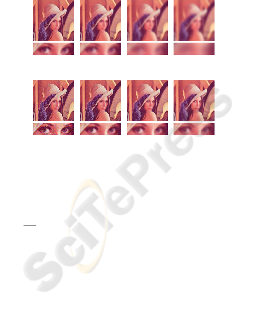
(a) (b) (c) (d)
Figure 1: Linear isotropic scale space for the Lena image: (a) c=1, (b) c=3, (c) c=20 and (d) c=250.
(a) (b) (c) (d)
Figure 2: Anisotropic scale space for the Lena Image with 20% uncorrelated noise for each pixel in the input image: (a) Input
image, (b) c=3, (c) c=20 and (d) c=250.
3 DIFFUSION
3.1 Isotropic Diffusion
In the simpliest case we have a quadratic neighbor-
hood U
i
of a pixel i and symmetric weighting factors
w
i j
= w
ji
= 1. Eq. (4) then is simplified to
∂
∂ξ
(x,k)
P(ξ) = ξ
(x,k)
− ξ
(x,k)
0
+ c
∑
j∈U
x
(ξ
(x,k)
− ξ
( j,k)
) (10)
This is the classic case of isotropic linear diffusion.
The isotropic diffusion as well as anisotropic dif-
fusion with symmetric weights, i. e. w
i j
= w
ji
, was al-
ready used by us in the context of stereoscopic depth
estimation ((Hund, 2002), (Brockers et al., 2005)).
There, eq. (10) and eq. (6), respectively, were used
to eliminate the ambiguities in the stereoscopic dis-
parity space.
Fig. 1 demonstrates the linear isotropic diffusion
properties on the Lena image. With growing reg-
ularization parameter c the image is isotropically
smoothed until all image detail is lost.
3.2 Anisotropic Diffusion
An important advantage of our problem formulation
in (2) is the fact that we are free to choose the weight-
ing factors w
i j
without loosing existence or unique-
ness of the solution. To achieve an anisotropic dif-
fusion behaviour, we use the following definition for
the local support area. The orientation angle associ-
ated with a pixel is derived by applying an orienta-
tion selective Gaussian based filterbank to the input
image. Due to the given orientation angle of a pixel
the coordinates of its eight-point neighborhood are ro-
tated into the coordinates (x,y) and the corresponding
weighting factors w
i j
are determined from the follow-
ing function
f (x,y) =
(
0 for y > 0.7
1.0 + cos
π · y
0.7
else
(11)
Eq. (11) ensures a strict diffusion along one direction.
For a more generous behaviour, the constants 0 and
0.7 in eq. (11) have to be changed. It is clear that
Q
i
=
1
2
∑
k
(w
ik
+ w
ki
) < Q in eq. (9) and hence eq.
(11) is well posed.
Fig. 2 demonstrates the anisotropic case on the
Lena image. This time, 20% uncorrelated noise is
ANISOTROPIC DIFFUSION BY QUADRATIC REGULARIZATION
103
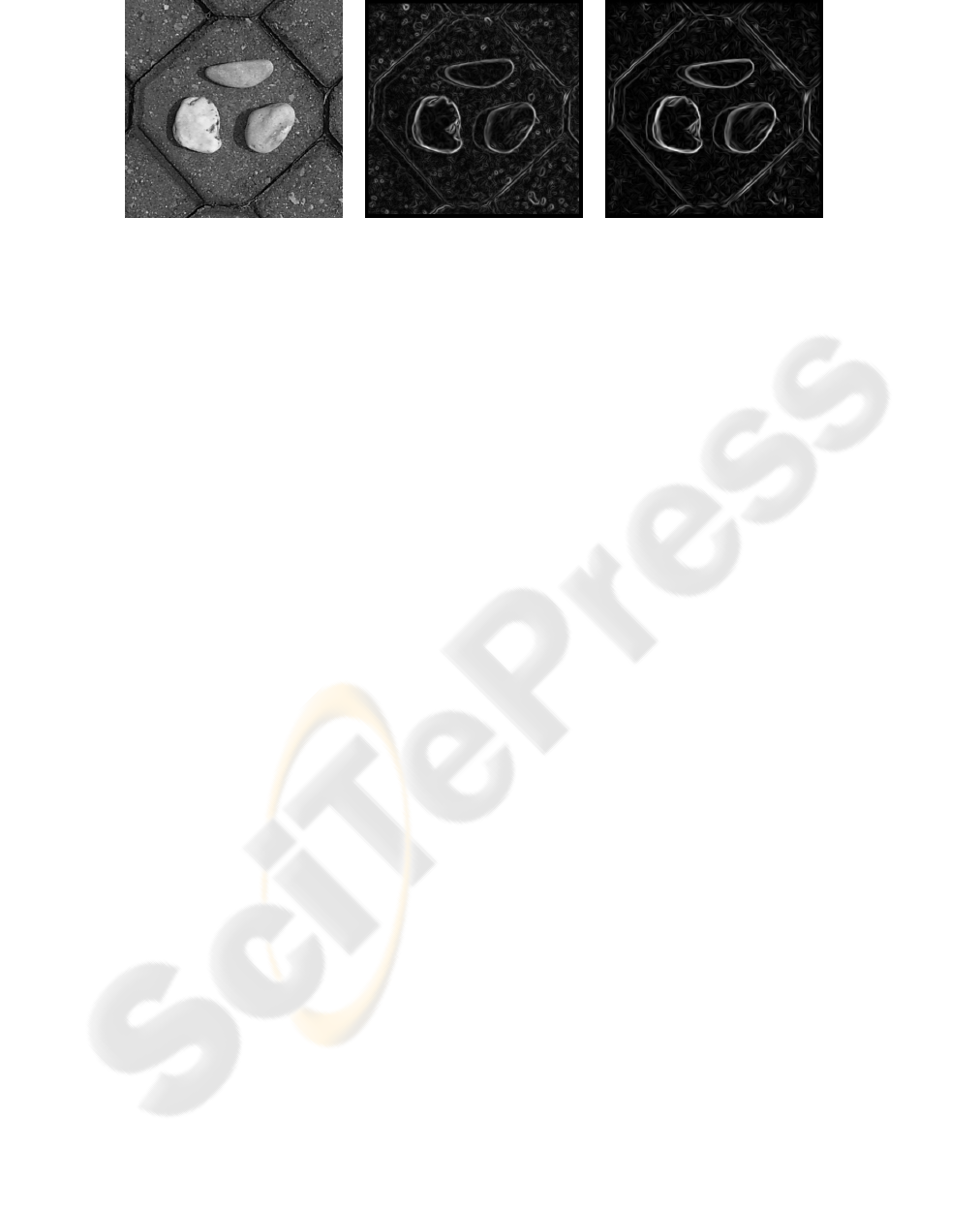
(a) (b) (c)
Figure 3: Stones image: (a) Input image, (b) gradient magnitude |∇g
x
| before and (c) after self-organization of the edge map.
added to each pixel of the input image. It becomes
obvious that for c → ∞, unlike in the linear isotropic
case, a local neighborhood can be defined for which
the method does not diffuse to a constant value for all
image pixels
4 MODIFICATIONS
4.1 Self-Organization of the Edge Map
As it is mentioned above, we use a Gaussian based
filterbank to derive the orientation angle we need to
determine the weighting factors w
i j
. Unfortunately
gradient based filters are very sensitive to noise.
In order to overcome this problem, we apply the
anisotropic regularization to the edge map that is gen-
erated by the Gaussian based filterbank, i. e. we ap-
ply eq. (2) for d = 2 to the edge map that is defined
by (ξ
(x,1)
,ξ
(x,2)
) = |∇g
x
|(cos(α
x
),sin(α
x
)) with |∇g
x
|
being the gradient magnitude and α
x
the associated
orientation at image position x.
During the iterative process, eq. (2) is reformu-
lated for each iteration step, since the weighting fac-
tors depend on the edge values that are modified. That
is, the orientation of an edgel determines the weight-
ing factors, that are used for one iteration step. This
step changes the edgel and therefore its orientation.
This leads to a self-organization of the edge map, en-
hancing salient contours. Note that this proceeding no
longer guarantees the uniqueness, the iteration con-
verges to a solution that depends on the starting vec-
tor. Nevertheless, regarding the numerical implemen-
tation in section 2.2 the convergence of the iteration is
still given since ρ(M) < 1. Furthermore, the problem
formulation for the image itself stays the same and
hence keeps the uniqueness property. Fig. 3 shows
the effect of a self-organizing edge map. High fre-
quencies in the input image Fig. 3(a) take effect on
the gradient-based edge map in Fig. 3(b). Applying
the self-organizing scheme emphasizes “important“
edges. This is also of interest for the topic of salient
contour inference, see (Mahamud et al., 2003) for ex-
ample.
4.2 Thresholding the Weighting Factor
To achieve an enhancement of discontinuities along
edges the weighting factors can be set to zero for
neighboring image elements i, j with |ξ
(i,k)
−ξ
( j,k)
| <
s for some threshold s. Note that again uniqueness is
lost and the result is highly dependent on the starting
vector ξ
0
. A good choice for ξ
0
is zero or a smoothed
version of the input image. For ξ
0
= ξ
0
and a small
threshold merely no effect will take place even for a
high smoothing factor.
5 EVALUATION
5.1 Qualitative Evaluation
The images in Fig. 4(a)-(d) are introduced in (Weick-
ert, 1996) as an example for the denoising properties
of different diffusion filters. 70% of the input image
in Fig. 4(a) are degraded by noise. Fig. 4(b) shows
the linear and (c) the nonlinear isotropic case while
Fig. 4(d) is computed with the proposed edge enhanc-
ing anisotropic diffusion approach.
In Fig. 4(f) the orientational approvement of the self-
organizing process we suggested in section 4.1 can
be seen compared to the initial values in Fig. 4(e)
that are received from an orientation selective, gaus-
sian based filter. Fig. 4(g) shows the solution of
the regularization term proposed in section 2.1 with
anisotropic weighting factors derived from the self-
organized edge map. Fig. 4(h) shows the same setting,
but with thresholded weighting factors. To achieve
VISAPP 2008 - International Conference on Computer Vision Theory and Applications
104
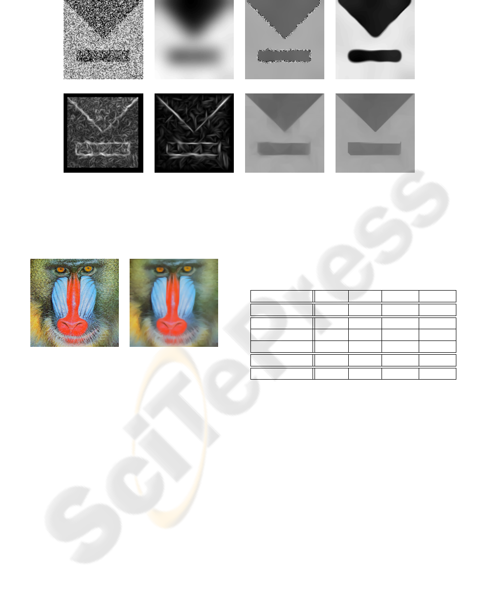
(a) (b) (c) (d)
(e) (f) (g) (h)
Figure 4: Images (a)-(d) taken from (Weickert, 1996) and (J
¨
ahne, 2002) respectively: (a) Input image, (b) linear diffusion,
(c) nonlinear isotropic diffusion and (d) nonlinear anisotropic diffusion. Images (e)-(h) demonstrate our approach: (e) Gradient
magnitude, (f) gradient magnitude after self-organization of the edge map, (g) result for the anisotropic diffusion proposed in
section 3.2 and (h) result with thresholded weighting factors.
(a) (b)
Figure 5: Mandrill image: (a) N - input image with 10%
uncorrelated noise and (b) R
250
n
- anisotropic diffusion with
c = 250.
maximal diffusion, the scale parameter in both cases
was set to c = 1000. As can be seen in the results
our algorithm shows a good noise elimination prop-
erty with a significant improvement in edge preserv-
ing.
5.2 Quantitative Evaluation
The results presented in table 1 are computed on the
mandrill image in Fig. 5(a) with 10 percent noise
added to each pixel of the input image. To compare
two images we take the percentage of pixels with an
absolute difference less than a threshold s compared
to the total number of pixels m · d. For a smoothness
factor c the result computed on the noisy input im-
age N is given by R
c
n
. Table 1 shows the similarity
between R
c
n
and the original image O.
Table 1: Mandrill image: similarity between noisy image
(N), original image (O) and computed images (R
c
).
Similarity s = 1 s = 6 s = 16 s = 21
N ∧ O 6.19 36.38 79.41 90.36
R
0.1
n
∧ O 4.04 40.88 85.60 94.40
R
0.3
n
∧ O 3.99 41.13 84.40 92.75
R
0.5
n
∧ O 3.90 40.24 81.75 90.29
R
0.1
l
∧ O 3.90 40.16 83.14 91.92
R
250
n
∧ R
250
o
29.18 98.83 99.97 99.99
Due to the high frequent image content in the orig-
inal image the diffusion process yields high similarity
values only for small smoothness factors. These re-
sults show a higher similarity to the original image.
than the noisy input image does. Of course, they also
show a higher similarity than an linear isotropic fil-
tered image (R
0.1
l
). On the other hand it can be seen
that for a large scale the diffusion process comes to
similar results when the original image is taken as the
input image (R
250
o
) as well as when the noisy image
is taken as the input image (R
250
n
). This shows that
unoriented noise as well as high frequent unoriented
image information is eliminated from the input image.
To our knowledge, the noise removal method pro-
posed in (Portilla et al., 2003) and (Guerrero-Colon
and Portilla, 2005) respectively is the most accurate
one. We therefore compare our results to those given
in (Portilla et al., 2003). Here, the denoising perfor-
mance is measured with the peak signal to noise ra-
ANISOTROPIC DIFFUSION BY QUADRATIC REGULARIZATION
105
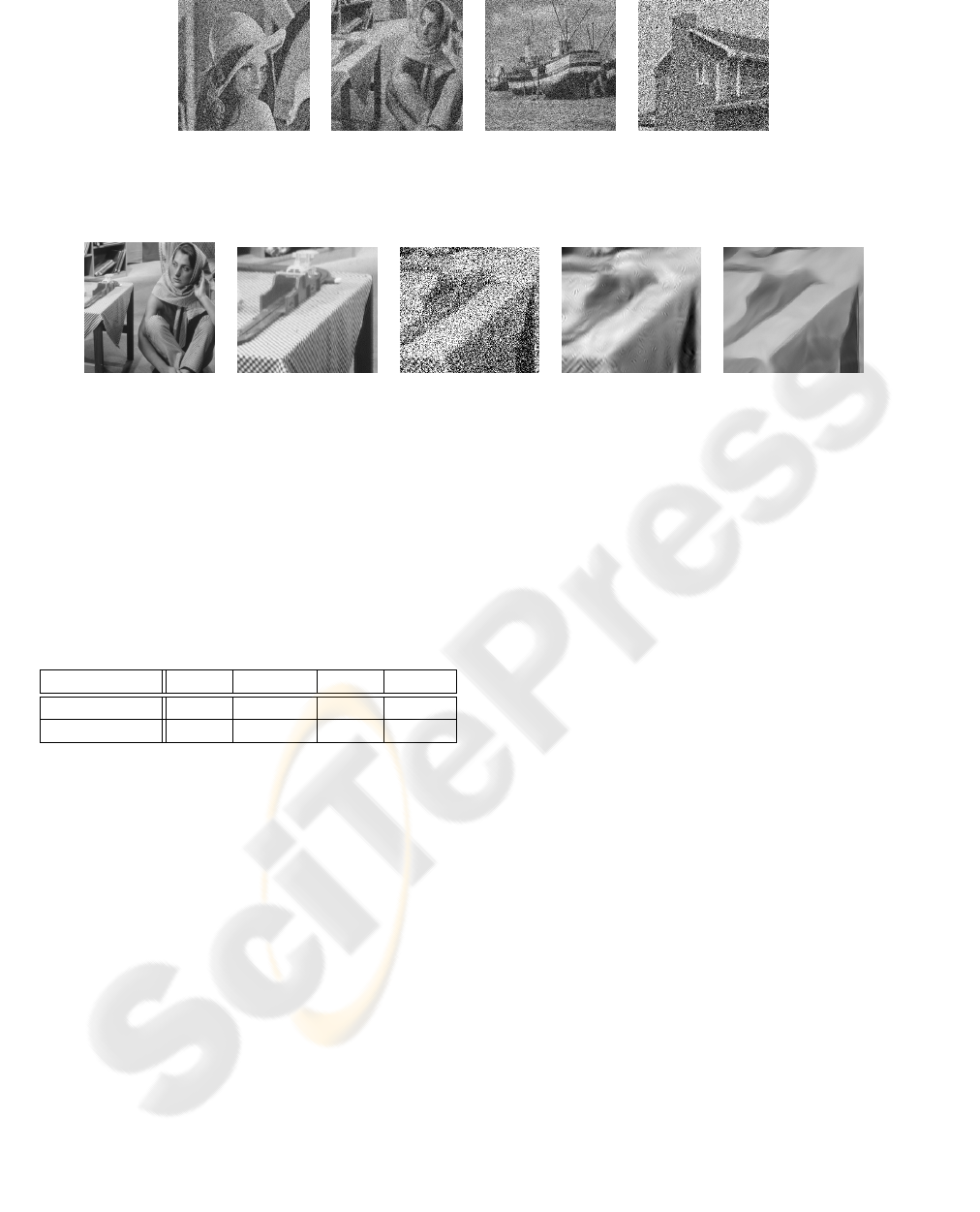
(a) (b) (c) (d)
Figure 6: Images used for evaluation in table 2: (a) Lena, (b) Barbara, (c) Boats and (d) House. The input images are degraded
with additive Gaussian white noise. All images are taken from http://decsai.ugr.es/ javier/denoise/
(a) (b) (c) (d) (e)
Figure 7: Barbara image: (a) original image, (b) magnification of the table region, (c) part of noisy input image with σ = 100
and PSNR = 8.13, (d) denoising result of Portilla et al. (PSNR = 22.6) and (e) denoising result of our method (PSNR = 22.1).
Table 2: Comparison of our denoising results with the re-
sults of Portilla et al., the results are expressed as peak
signal to noise ratio (PSNR). The input images, which are
shown in Fig. 6, are contaminated with additive Gaussian
white noise (σ = 100). The parameters of our method are
tuned to show best performance on the Lena image. All
images are computed with the same parameters.
σ = 100 Lena Barbara Boats House
Portilla et al. 25.64 22.61 23.75 25.11
Our method 25.65 22.07 23.13 24.92
tio PSNR = 20log
10
(255/σ
e
) with σ
e
being the er-
ror standard deviation. Looking at the PSNR val-
ues our method reveals a notable disadvatage. The
smoothing, especially for large smoothness factors,
leads to a shrinkage of the histogram. For the sake
of comparability, we therefore applied a linear his-
togram equalization on our results, but, as can be seen
in Fig. 7(e), there still remains a systematic deviation
of a regions greyscale level compared to the original
image (Fig. 7(b)). Our results are computed with a
smoothing factor c = 4.0 and 60 iteration steps. The
starting vector is the noisy input image and in a pre-
processing step, we perform the self-organization of
the edge map as it is described in section 4.1. For the
self-organization, we used a smoothing factor c = 8.0.
As can be seen in table 2, except for the Lena im-
age, our approach is outperformed by the method pro-
posed in (Portilla et al., 2003). Nevertheless it can be
observed that for high noise levels, our method pro-
duces less artifacts, which can be a crucial issue, not
only for subsequent image processing steps, but also
for the viewers subjective appraisement of the image
quality.
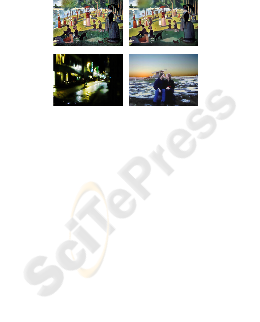
6 MORE RESULTS
Anisotropic diffusion processes also feature artistic
aspects. In (Weickert, 1996) , paintings of van Gogh
were used for coherence enhancing anisotropic dif-
fusion resulting in images that yield very different
impressions compared to the original paintings. In
Fig. 8(b) the anisotropic regularization we propose in
section 3.2 is used to eliminate the pointillism in a
painting of Georges Seurat (Fig. 8(a)). In Fig. 8(c)
and (d) the isotropic case in section 3.1 is combined
with the thresholding in section 4 and an oversmooth-
ing of the images in order to alienate the original im-
ages.
7 CONCLUSIONS AND
OUTLOOK
We presented a novel regularization-based approach
to anisotropic diffusion that provides a clear mathe-
matical formulation of the regularized diffusion prob-
lem and its solution. The solution is unique and the
iteration process to derive this solution is shown to
be convergent for any scale, i. e. smoothness factor.
VISAPP 2008 - International Conference on Computer Vision Theory and Applications
106
(a) (b)
(c) (d)
Figure 8: (a) Un dimanche apr
`
es-midi
`
a l’
ˆ
ıle de la grande jatte, 1884 (b) Result after applying anisotropic diffusion (c) Street
scene in Florence (d) Somewhere in Ireland.
The capability of our approach was demonstrated on
a variety of greyscale and color images. By our ap-
proach we hope to have closed a gap between classic
diffusion filters and regularization methods. Future
examinations will include verifying the rotation in-
variance properties of the local support area proposed
in section 3.2. Future work also will address the effect
of histogram shrinkage mentioned above and the im-
provement of the comparability of the noise removal
results.
REFERENCES
Aubert, G., Barlaud, M., Blanc-Feraud, L., and Charbon-
nier, P. (1997). Deterministic edge-preserving regu-
larization in computed imaging. IEEE Trans. Imag.
Process. 5(12).
Brockers, R., Hund, M., and Mertsching, B. (2005). Stereo
Matching with Occlusion Detection Using Cost Re-
laxation. In IEEE International Conference on Image
Processing (ICIP 2005), volume III, pages 389 – 392.
Guerrero-Colon, J. A. and Portilla, J. (2005). Two-level
adaptive denoising using gaussian scale mixtures in
overcomplete oriented pyramids. IEEE International
Conference on Image Processing (ICIP 2005), vol. I,
105-108.
Hund, M. (2002). Disparit
¨
atsbestimmung aus Stereobildern
auf der Basis von Kostenfunktionen. Diploma thesis,
University of Paderborn.
Ito, K. and Kunisch, K. (1999). An active set strategy based
on the augmented lagrangian formulation for image
restoration. M2AN Math. Model. Numer. Anal., Vol.
33, pp. 1-21.
J
¨
ahne, B. (2002). Digital image processing (5th ed.):
concepts, algorithms, and scientific applications.
Springer-Verlag.
Mahamud, S., Williams, L. R., Thornber, K. K., and Xu,
K. (2003). Segmentation of multiple salient closed
contours from real images. IEEE Trans. on Pattern
Analysis and Machine Intelligence, 25(4).
Nordstrom, K. N. (1989). Biased anisotropic diffusion–a
unified regularization and diffusion approach to edge
detection. Technical Report UCB/CSD-89-514, EECS
Department, University of California, Berkeley.
Perona, P. and Malik, J. (1990). Scale-space and edge detec-
tion using anisotropic diffusion. IEEE Trans. Pattern
Anal. Mach. Intell., 12(7):629–639.
Portilla, J., Strela, V., Wainwright, M., and Simoncelli, E.
(2003). Image denoising using scale mixtures of gaus-
sians in the wavelet domain. IEEE Trans. Image Proc.,
In Press. 2003.
Scharr, H. and Weickert, J. (2000). An anisotropic diffu-
sion algorithm with optimized rotation invariance. In
G. Sommer, N. Kr uger, C. Perwass (Eds.), Muster-
erkennung.
Weickert, J. (1996). Anisotropic diffusion in image process-
ing. Ph.D. thesis, Dept. of Mathematics, University of
Kaiserslautern, Germany.
Weickert, J. (1999). Coherence-enhancing diffusion of
colour images. Image Vision Comput., 17(3-4):201–
212.
ANISOTROPIC DIFFUSION BY QUADRATIC REGULARIZATION
107
