
ACCELERATED SKELETONIZATION ALGORITHM FOR
TUBULAR STRUCTURES IN LARGE DATASETS BY
RANDOMIZED EROSION
Gerald Zwettler, Franz Pfeifer, Roland Swoboda and Werner Backfrieder
Bio- and Medical Informatics Research Group, University of Applied Sciences Upper Austria, Campus Hagenberg
Softwarepark 21, A-4232 Hagenberg, Austria
Keywords: Morphological Operators, Fast Thinning, Skeletonization, Computer Aided Diagnostics.
Abstract: Skeletonization is an important procedure in morphological analysis of three-dimensional objects. A
simplified object geometry allows easy semantic interpretation at the cost of high computational effort. This
paper introduces a fast morphological thinning approach for skeletonization of tubular structures and objects
of arbitrary shape. With minimized constraints for erosions at the surface, hit-ratio is increased allowing
high performance thinning with large datasets. Time consuming neighbourhood checking is solved by use of
fast indexing lookup tables. The novel algorithm homogenously erodes the object’s surface, resulting in an
accurate extraction of the centerline, even when the medial axis is placed between the actual voxel-grid. The
thinning algorithm is applied for vessel tree analysis in the field of computer-based medical diagnostics and
thus has to meet high robustness and performance requirements.
1 INTRODUCTION
Thinning is the morphological process of removing
parts of a binary object’s surface until only the inner
core remains. The remaining object’s core is called
skeleton and should be aligned as close as possible
to the medial axis of the original object.
Continuous object surface removal is usually
accomplished with erosion and Hit-or-Miss
operators (Serra, 1982). Depending on thinning
constraints, side effects like foreshortening and
breaking of connections are prevented. Thinning for
2D data may be implemented following (Gonzales
and Woods, 2001) using Hit-or-Miss transformation,
iteratively applying eight structuring elements.
For thinning on three-dimensional input data,
Jonker (Jonker, 2002), (Jonker, 2004) presents a
thinning algorithm based on shape primitives for
space curves and surfaces. The approach uses Hit-
or-Miss transformations with a set of structuring
elements according to the dimensionality of the
input mask. The focus of their work lies on the
calculation of these structuring elements for
arbitrary dimensionality and neighbourhood
connectivity. When extracting an object’s skeleton,
shape primitives for space curves but also for space
surfaces must not be further eroded. With this
approach shape preserving thinning is guaranteed.
The algorithm is quite costly as Hit-or-Miss
transformation has to be performed for the entire
image mask with more than 50 million structuring
elements for 3D data. In the work of Lohou a Binary
Decision Diagram (BDD) is introduced for
combining these millions of structuring elements,
thus reducing complexity of the thinning algorithm
to 12 sub-iterations (Lohou, 2001).
As the novel thinning algorithm described in this
work is needed for centerline detection as pre-
processing for vessel graph analysis, no shape
preserving for arbitrary objects but a fast algorithm
is required, as large CT vessel data has to be
processed.
2 METHODS
2.1 Basic Notations
Thinning algorithms usually work on binary 3D
image data. The basic notations defined in this
section are basis for our thinning algorithm.
74
Zwettler G., Pfeifer F., Swoboda R. and Backfrieder W. (2008).
ACCELERATED SKELETONIZATION ALGORITHM FOR TUBULAR STRUCTURES IN LARGE DATASETS BY RANDOMIZED EROSION.
In Proceedings of the Third International Conference on Computer Vision Theory and Applications, pages 74-81
DOI: 10.5220/0001077000740081
Copyright
c
SciTePress

2.1.1 Binary 3D Object
Under the terms of set theory, a binary image A in
Ζ
3
is a set of n foreground elements a = (a
x
, a
y
, a
z
).
The following definition is established:
()
⎭
⎬
⎫
⎩
⎨
⎧
∈
=
else
Aaif
aforeground
0
1
:
.
(1)
Consequently, a voxel not contained in A belongs to
the complementary set of A, defined as background.
2.1.2 Morphological Operators
The two basic operations of Mathematical
Morphology, dilation and erosion, are defined as
(
)
{
}
≠= ABzBA
z
I
ˆ
|«
.
(3)
(){}
ABzBA
z
⊆= |x .
(4)
for voxels z in Ζ
3
with binary input image A,
structuring element B and the reflection of B
(Gonzales and Woods, 2001).
The morphological transformations of Equ. 3
and Equ. 4 can be expressed with Minkowski
addition and subtraction by the following equations
(Vincent, 1991), where b refers to the elements of
structuring element B and x refers to the elements of
the resulting set:
{
}
AbxBbxBA ∈−∈∃∈= ,|
3
A«
.
(5)
{
}
AbxBbxBA ∈−∈∀∈= ,|
Ax
.
(6)
Those formulations are adapted for Ζ
3
. Dilation and
erosion are typically implemented as kernel
operations (Gonzales and Woods, 2001). The hot-
spot of structuring element B translates over all
elements of A. In case of dilation, all elements of B
are set in the result, if the position under the hot-spot
in A is set too, see Equ. 5. Erosion only preserves
those parts of A where A and B fully overlap.
Many common image processing applications let
the user control the filtering process by the choice of
structure element’s shape and size rather than by a
specified number of iterations. Most complex
structure elements of large size may be decomposed
to simple structure elements of size three in each
dimension (Park and Chin, 1995), (Anelli et al.,
1996). This decomposition is efficient for arbitrary
structure elements. In the presented work only
simple 3D structuring elements are used, see Fig. 1.
Figure 1: Simple structuring elements for application of
morphological operators in 2D and 3D. 2D elements are
named as N
8
and N
4
(left) respectively as N
26
and N
6
for
the analogous ones in 3D (right).
Besides recursive decomposition to default
structuring elements, there is a further optimization
potential. When using a structuring element B for
morphological operation on A, it is sufficient to
apply B on the surface of A (Vincent, 1991),
elements with not all neighbours set in
N
26
.
Both, recursive application of structuring
element B and the constraint to operate on the
surface of A lead to an enormous reduction of
runtime as will be presented in the following
sections.
2.2 Hit-or-Miss Thinning
For a set A, thinning can be defined as Hit-or-Miss
transformation, defined in Equ. 7, for mask B with
foreground (B
set
, 1) and background (B
unset
, 0)
values.
(
)
)(
unsetset
BABABA « ª
−
x . (7)
The other positions in the structuring elements are so
called “don’t cares” (Jonker, 2002).
Thinning is defined as Hit-or-Miss
transformation on a set of structuring elements
B={B
1
, B
2
, … B
n
} and all rotated and mirrored
variants of B. Structuring elements for Hit-or-Miss
transformation not only define required foreground
positions but also required background positions to
perform erosion / dilation.
The Hit-or-Miss operation is iteratively repeated
until a convergence criterion is reached. Typically
convergence is reached when no single erosion is
performed for a full iteration cycle. If a voxel in A
under the hot-spot of mask B meets the Hit-or-Miss
condition, erosion can be performed (the concerning
voxel in A is labelled as hot-spot in the following
section).
Constraints for the skeleton are (a) constant
thickness of diameter one when convergence is
reached and (b) the prevention of connection
intersection. For an object fully connected in N
26
, the
skeleton must remain fully connected.
Furthermore thinning must prevent
foreshortening of the resulting skeleton. Therefore
ACCELERATED SKELETONIZATION ALGORITHM FOR TUBULAR STRUCTURES IN LARGE DATASETS BY
RANDOMIZED EROSION
75

erosion at the ends of skeletons with target thickness
of one must be avoided.
Figure 2: Input object and resulting skeleton. The skeleton
remains fully connected. No foreshortening at the endings,
i.e finger tips (Jonker, 2004).
2.3 Accelerated Thinning
The developed thinning algorithm can be iteratively
applied on the object’s surface for preserving a
centerline of good quality in minimal time. Only
homogenously applied in-place erosion with default
structuring element N
6
is needed to calculate the
centerline of a binary tubular object A, when the
surface is homogenously eroded from all directions.
The critical point is how to erode in such a uniform
way that the correct centerline is extracted.
To preserve fully-connectedness, erosion of the
hot-spot is only valid, when it is not the only
connection between the vessel elements in N
26
around the hot-spot. Otherwise connections break
and convergence is reached when the object mask
has totally disappeared. Further erosion at the end of
the “tail” is not performed to prevent continuous
shortening of the resulting vessel centerline.
Providing the correct centerline location, not all
elements of the surface are considered for erosion.
Only those voxel positions with a “low” number of
set neighbours in N
26
are taken into account for
erosion as they belong to the “outer” surface.
Without this restriction erosion along the
centerline’s orthogonal plane is enforced resulting in
a misplaced centerline.
2.4 Algorithm Description
Neighbourhood conditions for dilation on the
surface of an object are introduced to preserve
connections and to ensure total erosion of the object.
For each N
26
check, only the hot-spot is considered
for erosion operation.
2.4.1 First Neighbourhood Condition
Two voxel i and j are neighbours in N
26
when their
position Δ in all dimensions k is one voxel width at
the most, see Equ. 8.
Whenever the hot-spot is set in a N
26
neighbourhood, all set neighbours (defined in Equ.
8) are fully-connected at least via the hot-spot
position, as the hot-spot is neighbour of all other
elements in N
26
, see Equ. 10. When eroding the hot-
spot, the remaining elements in N
26
must remain
fully connected and thus preventing break-up of
connected structures, see Equ. 11. Fig. 3.a shows
neighbourhood configurations, where erosion of the
hot-spot would lead to a break-up of connectivity.
The hot-spot in the neighbourhoods visualized in
Fig. 3.b are valid for erosion of the hot-spot
concerning the first neighbourhood condition.
.
1),(),(:
0
1
:),(
1
⎪
⎭
⎪
⎬
⎫
⎪
⎩
⎪
⎨
⎧
≤−∀
=
=
kjidxkiidx
else
if
jinb
D
k
(8)
(
)
(
)
.
),(),(:),(
0
1
:),(
⎭
⎬
⎫
⎩
⎨
⎧
∧∃∨
=
jkconnkinbkjinb
else
if
jiconn
(9)
.
),(),(:,
0
1
:)(
⎭
⎬
⎫
⎩
⎨
⎧
∨≠∀∀
=
∈∈
jiconnjinbji
else
if
NfConn
DD
NjNi
D
(10)
()
()
(
)
.
0
1
:1
⎭
⎬
⎫
⎩
⎨
⎧
−
=
DD
D
NhotSpotNfConn
else
if
NnCond
(11)
2.4.2 Second Neighbourhood Condition
Erosion of the hot-spot is prohibited when it leads to
foreshortening of the thinned object. At a number of
only three remaining set elements in the
neighbourhood, no further thinning of this area is
required, see definition in Eq. 12. Examples for
these neighbourhood configurations are shown in
Fig. 3.c.
()
(
)
.
0
1
:,2
⎭
⎬
⎫
⎩
⎨
⎧
>
=
lNsize
else
if
lNnCond
D
D
(12)
Combining the first and second neighbourhood
condition, erosion of the hot-spots is driven until a
convergence criterion is reached and no valid
erosion operations are identified for an entire
iteration step. Implying the first two neighbourhood
conditions, erosion still has to be restricted to the
object’s surface, introducing the third condition.
2.4.3 Third Neighbourhood Condition
The hot-spot in Fig. 3.d is per definition part of the
current object’s surface. In those cases, however,
erosion would lead to a grabbing into the object that
negatively influences the centerline shape and
position. Consequently, the definition for surface has
to be restricted. Analyzing the object’s surface area,
no neighbourhood configurations are obvious with
more than 12 neighbours besides the hot-spot and
VISAPP 2008 - International Conference on Computer Vision Theory and Applications
76
the hot-spot being interpreted as part of the “outer”
surface (see Equ. 13). A voxel is element of the
“outer surface” when there is at least one
background neighbour in N
6
.
Note that raising the background neighbour
threshold from base level 12 leads to an increase in
runtime but a reduction of side-effects concerning
quality of the resulting centerline. The gain in
performance for use of larger threshold values result
from the higher number of erosions (higher hit-ratio)
that can be performed during each iteration step.
Experimental tests showed that the quality of the
thinning results is hardly affected up to a threshold
level of 15 but runtime is reduced due to a higher
percentage of erosions performed for the time-
consuming neighbourhood checking. Nevertheless,
this threshold parameter can be used to balance
between quality and runtime.
All three conditions must be met to erode the
hot-spot position, see Equ. 14.
()
()
.
0
1
:,3
⎭
⎬
⎫
⎩
⎨
⎧
<
=
uNsize
else
if
uNnCond
D
D
(13)
()
()
[]
()
() ( )
.
,3,2
1
0
1
:,,
⎪
⎭
⎪
⎬
⎫
⎪
⎩
⎪
⎨
⎧
⎟
⎟
⎠
⎞
⎜
⎜
⎝
⎛
∧
∧∧
=
uNnCondlNnCond
NnCondNhotSpotN
else
if
ulNerode
DD
DDD
D
(14)
2.5 Mapping of Neighbourhood
Conditions
Neighbourhood conditions 1 and 2 lead to an overall
number of 5,421,509 configurations in N
26
where
erosion of the set hot-spot is not allowed. Compared
to the total number of different configurations in N
26
with a set hot-spot, namely 67,108,864 (2
26
), only in
8.08% of all cases erosion is not allowed.
Checking the neighbourhood around each hot-
spot for fulfilling the neighbourhood criterions
during the thinning operation is too time-consuming
from an implementation point of view. Instead, a
mapping for all possible configurations in N
26
is pre-
calculated. All possible 2
26
configurations are
generated and checked for the neighbourhood
criterions. The boolean result is persisted to a file as
lookup table. The applied mapping code is derived
from the neighbourhood configuration. Each
position in N
26
neighbourhood is coded as a defined
bit-position in the 2
26
hash code, where position 0 is
coded as bit 0, position 1 as bit 1 and so on.
Generation of the lookup-file takes about 3 minutes
performed on Intel Pentium 4 with 2.8GHz. Note
that this has to be executed only once.
When iterating over the voxels of object A, the
calculation of the hashing code is the only operation
to perform. Direct mapping with the neighbourhood
configuration code leads to a boolean value
indicating whether erosion is allowed or not for
current neighbourhood configuration.
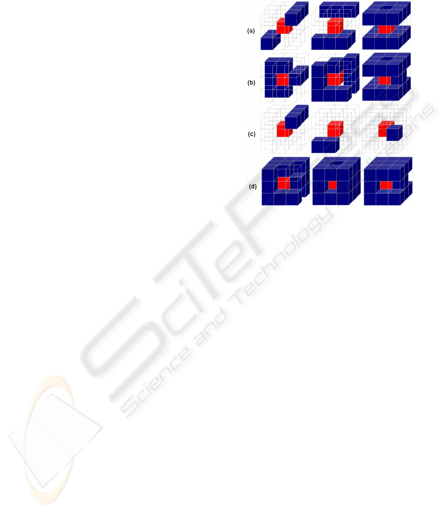
Figure 3: Neighbourhood configurations where erosion of
the hot-spot is allowed or permitted. Upper row (a):
erosion would lead to loss of full-connectivity as the other
neighbours would get separated when the hot-spot is
removed. Row (b): erosion would not influence
connectivity and therefore is allowed as the remaining
neighbours are still fully-connected. Foreshortening of the
skeleton has to be prevented in (c). Lower row (d):
Although the hot-spot is part of the surface, erosion would
cause grabbing into the object, that has to be prevented by
applying neighbourhood condition 3 (Equ. 13).
2.6 Balanced Surface Erosion
The erosion order for the object voxels is important
for the symmetry of the extracted medial axis.
Continuous iteration as well as recursive
propagation would strongly prefer elements at the
beginning and thus yields a deviation of the resulting
skeleton from the optimal medial axis, depending on
the propagation order and direction. To overcome
this inadequacy, random neighbourhood selection is
applied. Balanced erosion from all sides of the
object leads to significant improvements. The
described random shuffling has to be performed only
once for initialization of the processing order.
Only the surface elements with at least one
background neighbour are relevant at each iteration
step. Hence for each iteration run, only these surface
elements are taken into consideration. Using a
structuring element B for morphological operations
ACCELERATED SKELETONIZATION ALGORITHM FOR TUBULAR STRUCTURES IN LARGE DATASETS BY
RANDOMIZED EROSION
77
on A it is sufficient to apply B only on the surface of
A (Vincent, 1991), more precisely all elements with
at least one background neighbour set in
N
26
.
When eroding a certain voxel, all of it’s
foreground neighbour voxels become elements of
the “outer” surface. This way, a homogenous erosion
of the surface is ensured for arbitrary shaped objects.
Constriction of the morphological erosion to
surface voxels leads to a significant reduction of
runtime complexity, as discussed in the results
section.
2.7 Post-Processing
The presented method yields centerlines aligned as
much as possible along the middle of the tubular
object, but that very likely do not build up a straight
line. This results from the random iteration order
described before. The linearity of results primarily
depends on the objects size. For a symmetric
ellipsoid of size 10x10x100 used as test data, there is
e.g. no discrete course of connected points
representing the centerline. Consequently, the
resulting centerline’s voxel are aligned at discrete
positions around the optimal course, see Fig. 7.b.
Other centerline approaches (Jonker 2004) would
lead to a straighter result, but differing from the
optimal center according to the preferred
segmentation direction.
Results of the thinning algorithm can be further
smoothed using interpolation. To preserve hierarchy,
cyclic graph creation has to be applied for vectorized
centerlines. The voxels along the graph’s edges are
smoothed by interpolation-techniques. This post-
processing strategy with vectorization and graph
creation is presented in (Zwettler et al., 2006) for
acyclic 2D vessel data and can be analogously
expanded to application on three-dimensional data.
3 RESULTS
When performing erosion and dilation operations
with decomposed structuring elements on the
object’s surface, a significant gain in performance is
achieved. In Fig. 4 surface based dilation with
minimal size of structuring element B is presented.
Tab. 1 and Tab. 2 illustrate results of
performance analysis on dilation algorithms for the
input mask discussed in Fig. 4. Algorithm M1 uses a
large structuring element of size 7x7 translated over
the entire image mask. For M1’ translation is
restricted to the outer surface. M2 algorithm
decomposes the large structuring element to several
iteration steps with a default structuring element, see
Fig. 4.a. For M2’ the decomposed structuring
element appliance is restricted to the object area and
for M2’’ restricted to the object’s surface.
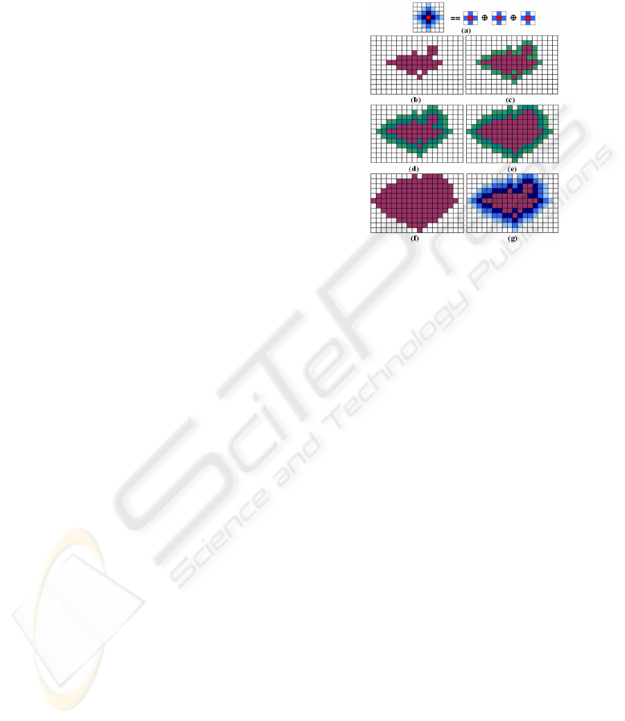
Figure 4: The shown structuring element of size 7x7 is
decomposed to three iterations using N
4
(a). Three dilation
iterations (c-e) on input mask (b). Only elements of the
surface vector are used for morphological operations.
Changes of current iteration are stored in the surface
vector used during next iteration. The iterative approach
and the usage of large structuring element result in the
same output masks (f-g).
Results of algorithm complexity measures show
a significant increase for iterative and surface based
dilation. The improvement increases with the size of
the binary object in relation to the entire mask size.
Runtime complexity for M1, M1’, M2, M2’ is
(
)
nheightwidthO
⋅
⋅
with n as the number of iterations,
respectively the size of structuring element B.
Runtime complexity can be approximated for M2’’
with
(
)
(
)( )
heightwidthrnrOnrO ,min,2 ≤
⋅
≅
⋅
⋅
⋅
π
for
a fixed radius. Similar findings concerning runtime
analysis are presented in Tab. 5 for 3D data and in
the work of Nikopoulos for surface based
morphological operations (Nikopoulos and Pitas
2000). The improvement depends on the volume-to-
surface ratio of the object.
Further runtime analysis is evaluated for 3D
dilation, see Tab. 3. Comparing results in row 1 with
2 (n=1 and n=4) and 3 with 4 (n=10 and n=20) for
M2’’, linear time complexity is observed whereas all
other approaches approximately have square
complexity concerning number of iterations n.
VISAPP 2008 - International Conference on Computer Vision Theory and Applications
78
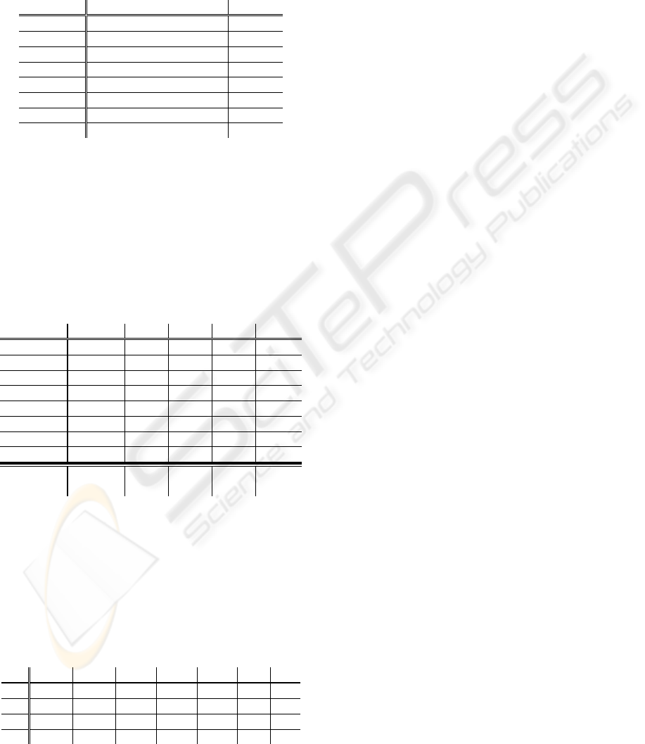
Table 1: Arithmetic operations used for decomposition of
the dilation algorithm. Weight value classification for
basic operations are based on runtime analysis of
(Blaschek, 2007) executed for integer operations on
Pentium IV, 2.4 GHz; code compiled with Microsoft
Visual C++ 7.1. Index operation weight composition is
defined according to results of performed runtime
analysis.
operation description weight
Op1 2D index calculation 4.4
Op2 2D index access 17.3
Op3 value comparison 6.4
Op4 mapping index calc. 107.6
Op5 value assertion 1.0
Op6 1D index calculation 2.2
Op7 1D index access 3.3
Op8 1D vector element add 4.3
Table 2: Runtime complexity of several dilation
approaches evaluated for 2D example presented in Fig. 2
(b). Number of executions for the basic operations [1-8]
described in Tab. 1 are listed. M1: large structuring
element translated over entire mask. M1’: large structuring
element translated over surface. M2: iterative applying of
small structuring element over entire mask. M2’: iterative
applying on binary object structure. M2’’: iterative
applying on surface. Total weight is calculated from
number of executions listed in Tab. 2 and weights listed in
Tab. 1.
operation M1 M1’ M2 M2’’ M2’’’
Op1 1955 240 2457 1977 240
Op2 2830 1115 2457 1977 240
Op3 2830 1115 2457 1977 1190
Op4 875 875 965 965 470
Op5 875 875 965 91 91
Op6 0 35 0 126 655
Op7 0 35 0 126 655
Op8 0 35 0 126 287
weight /
1000
170.7 122.9 173.8 160.7 68.3
Table 3: Runtime analysis on binary results of liver
segmentation at different number of iterations; Presented
values are the execution time in seconds. Data set size:
280x233x318. segmented volume: 4,689,190 voxels
(22.6%) initial surface: 283,925 voxels (1.4%). Runtime
test performed on Intel Pentium 4, 2.8GHz. P1: execution
with MeVisLab (http://www.mevislab.de/); P2: execution
with insight toolkit’s (ITK) (http://www.itk.org/)
itkBinaryDilateImageFilter integrated into MeVisLab
networks.
n M1 M1’ M2 M2’ M2’’ P1 P2
1
1.17 0.47 0.87 0.87
0.06
15.1 38
4
17.09 1.53 3.76 3.55
0.24
50.2 150
10
168.2 11.90 10.03 10.57
0.61
102 378
20
1808 119.9 22.33 25.40
1.26
199 757
Quality and performance of the presented thinning
method is demonstrated on the basis of several tests
with data at different scale. Further the hit-ratio, i.e.
the number of performed erosions divided by the
total number of neighbourhood checkings, is
emphasized as measure for thinning algorithm
efficiency. Validation of the resulting centerline is
performed by measurements on the centerline’s
position, see Tab. 4.
Depending on the volume-to-surface ratio, the
restriction of the presented fast thinning algorithm
for the total object (FT) on the object’s surface
(FT_surf) goes along with an increased hit-ratio.
FT and
FT_surf lead to different skeletons, as
FT morphology is performed in-place and because
changes influence the neighbourhood of voxel not
examined during the current iteration. On the other
hand
FT_surf only processes all surface elements
during each iteration what leads to more
homogenous results compared to FT.
The center of mass Δ in Tab. 4 refers to the level
of misplacement. For presented test data with even
dimensions, no discrete centerline is calculated.
Hence an error far below an Euclidian voxel
distance of 0.5 constitutes an improvement over
thinning algorithms that would result in a more
linear centerline at the cost of an exact misplacement
Δ of 0.5 depending on the preferred operation
direction, see (Jonker, 2002).
The resulting centerlines of the test runs logged
in Tab. 4 are plotted in Fig. 5 and 6 and visually
presented in Fig. 7-10.
As shown in Fig. 4, FT_surf leads to a
significant reduction in runtime compared to
Jonker’s implementations, with regard to the
increased hit-ratio. The correlation of FT after
square rooting confirms the stated reduction of
runtime complexity when restricting morphological
operations to the object’s surface.
To receive objective results, the implementations
for the Jonker approaches and FT_surf are
implemented as similar as possible. The typically
recursive implementation of Jonker (J_rec) shows
longer runtimes than the iterative implementation
(J_iter) analogously derived from our thinning
approach with Jonker’s structuring elements. Of
course they also feature the fast surface erosion in
contrast to FT. Reduction of runtime mainly results
from a more effective hit-ratio, see Fig. 6. For
FT_surf only 5,421,509 (8.08%) of all
configurations are rejected for erosion, whereas
Jonker’s space curve and surface shape primitives
lead to more than 34 million (~53%) rejections.
ACCELERATED SKELETONIZATION ALGORITHM FOR TUBULAR STRUCTURES IN LARGE DATASETS BY
RANDOMIZED EROSION
79
Results of thinning a volumetric ellipsoid are
presented in Fig. 7. The remaining skeleton is fully-
connected and positioned around the virtual rotation
center. Jonker’s algorithm results in a straighter line
with a Δ of about 0.5 from the rotation axis.
FT_surf is adequate for center detection of a sphere,
see Fig. 8.
Table 4: Results of thinning algorithm test runs on data
with different tubular and rotation-symmetric morphology.
The erosion percentage refers to the number of erosions
compared to all neighbourhood checkings. Erosion
percentage is significant for the performance increase that
can be seen comparing FT and FT_surf, the presented
thinning algorithm applied to the object’s surface.
[Runtime test performed on Intel Pentium 4, 2.8GHz].
ellipsoid, 40x40x400, voxel: 335,232; surface: 50,904
J_iter J_rec FT FT_surf
iterations 43 21 158 40
hit-ratio 0.986 0.949 0.019 0.988
time [sec] 0.876 1.919 19.641 0.671
centerline
length
394 385 379 395
center o
f
mass Δ
.48 .5 .0 .46 .5 3.02 .06 .09 .17 .03 .03 .4
ellipsoid, 80x80x800, voxel: 2,681,050; surface: 207,336
J_iter J_rec FT FT_surf
iterations 93 41 342 84
hit-ratio 0.99 0.958 0.009 0.981
time 6.214 24.27 402.36 4.962
centerline 784 781 837 770
center o
f
mass Δ
0.54 0.48
1
0.47 0.5
8.8
.02 .07 6.2 0.01 0.04 5
sphere, 200x200x200, voxel: 4,188,900; surface: 186,176
J_iter J_rec FT FT_surf
iterations 399 101 427 206
hit-ratio 0.984 0.926 0.008 0.991
time 13.492 70.98 721.41 6.117
centerline 389 174 3 3
center o
f
mass Δ
15.4 22
25.1
66 30 67 .17 .5 .17 0.17 0.17
0.5
grid, 200x200x200, voxel: 4,288,580; surface: 1,091,381
J_iter J_rec FT FT_surf
iterations 122 20 559 63
hit-ratio 0.697 0.511 0.005 0.774
time 14.243 40.011 1160.0 7.599
centerline 39,934 39,642 33,645 34,476
vessel tree, 318x316x454, voxel: 146,783; surface: 70,418
J_iter J_rec FT FT_surf
iterations 68 15 66 86
hit-ratio 0.443 0.308 0.064 0.484
time 1.096 3.601 11.578 0.890
centerline 3,595 3,506 3,385 3,692
Skeletonization of a three-dimensional grid confirms
that all object connections remain fully connected,
see Fig. 9.
The extraction of a vessel tree centerline is
demonstrated in Fig. 10. Results are suitable for later
vessel tree vectorization, cyclic graph creation and
graph analysis.
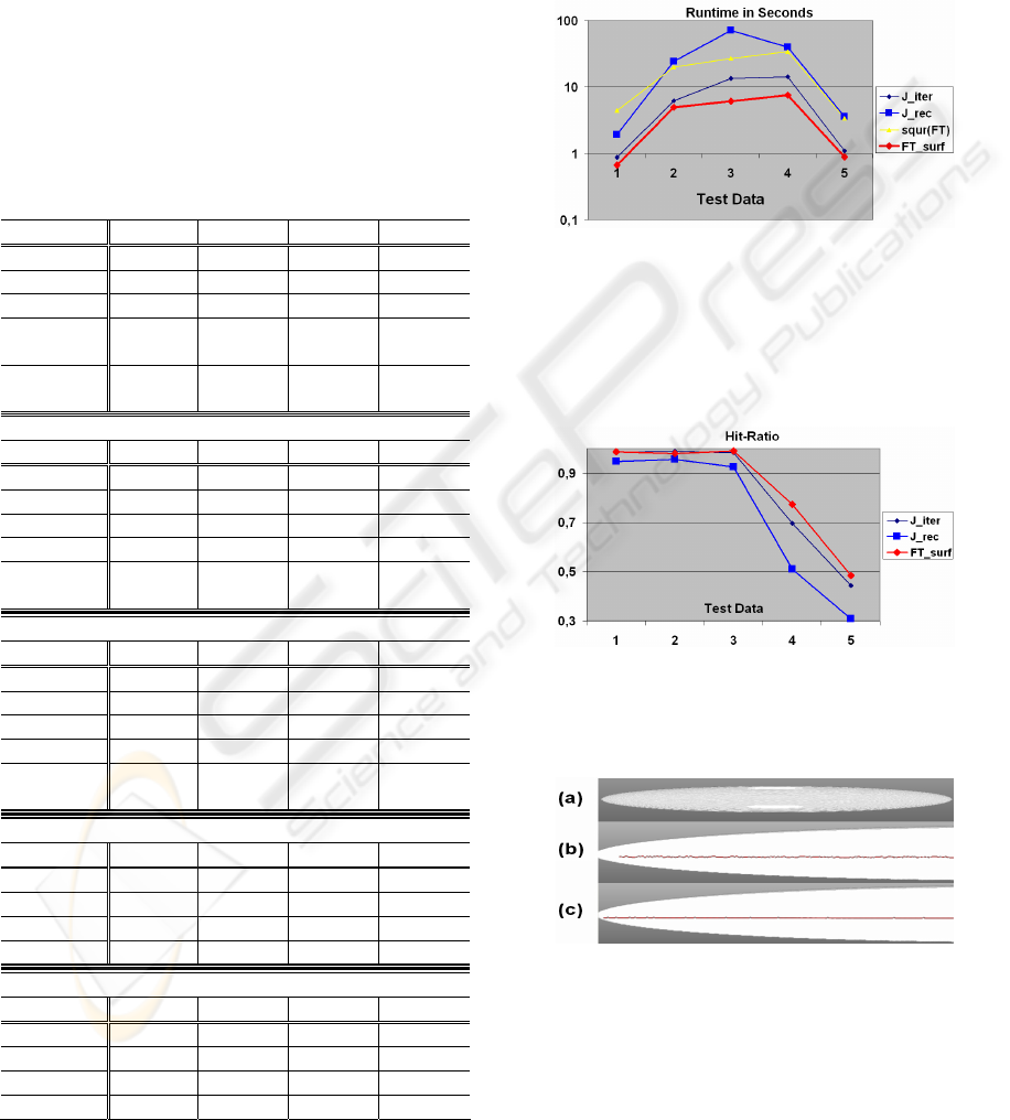
Figure 5: Results of runtime analysis presented in Tab. 4.
FT_surf shows lowest runtime for all 5 test data sets. FT,
the only approach not thinning at the object’s surface, was
plotted after square rooting. Evidently, erosion
constriction to the surface voxels leads to an approximated
runtime reduction by one dimension as stated for 2D data
in the section before.
Figure 6: Hit-ratio analysis based on test runs presented in
Tab. 4. The marginal hit-ratio improvements of FT_surf
compared to the Jonker implementations lead to a
significant reduction in runtime.
Figure 7: Thinning of an ellipsoid (a). Results of FT_surf
presented in (b) and results of J_rec in (c) (zoomed sub-
section).
VISAPP 2008 - International Conference on Computer Vision Theory and Applications
80

Figure 8: Thinning of sphere (a). FT_surf detects center
of the sphere as hot-spot (b) whereas inhomogeneous
erosion can lead to branched results (c), a side effect of
many other thinning algorithms.
Figure 9: Thinning of a 3D grid (a). Results of FT_surf
presented in (b) and (c).
Figure 10: Thinning of hepatic vessel tree (a). Results
presented in (b), (c) and zoomed vessel branching in (d).
4 CONCLUSIONS
In this paper existing algorithmic concepts for
acceleration of morphological operations are
combined for development of a novel thinning
concept optimized for the application area of tubular
structures. The presented algorithm is robust and fast
compared to other state-of-the-art thinning
operators, taking advantage due to the specialization
on tubular and rotation-symmetric morphological
objects.
The algorithm meets all requirements for clinical
application in the field of liver vessel graph analysis
for liver lobe classifications. As the presented
algorithm yields no favourite segmentation
direction, the resulting centerlines are closer to the
rotational axis when the object’s dimension is even
at the cost of generally not smoothed centerline
characteristics. The constraints of full-connectivity
and a centerline width of one are invariably fulfilled.
ACKNOWLEDGEMENTS
This work was supported by the project “Liver
Image Analysis using Multi Slice CT” (LIVIA-
MSCT) funded by the division of Education and
Economy of the Federal Government Upper Austria.
Special thank is given to PD Dr. Franz Fellner
and Dr. Heinz Kratochwill from the Central Institute
of Radiology at the General Hospital Linz for
valuable discussion.
REFERENCES
Anelli, G., Broggi, A., Destri, G., 1996. Toward The
Optimal Decomposition Of Arbitrary Shaped
Structuring Elements By Means of Genetic Approach.
In Mathematical Morphology and its Application to
Image and Signal Processing, pp. 227-234, Kluwer
Academic Publisher.
Blaschek, G.,2007. Algorithmen und Datenstrukturen 1
und Praktische Informatik. In Lecture Notes, Institut
for Pervasive Computing, University of Linz.
Gonzales, R.C., Woods, R.E., 2001. Digital Image
Processing. Prentice-Hall Inc., Upper Saddle River,
New Jersey, 2
nd
edition.
Jonker, P.P., 2002. Skeletons in N dimensions using shape
primitives. In Pattern Recognition Letters, vol 23, pp.
677-686.
Jonker, P.P., 2004. Discrete topology on N-dimensional
square tessellated grids. In Image and Vision
Computing, Vol. 23, Issue 2, 2005, pp.213-225.
Lohou, C., Bertrand, G., 2001. A new 3D 12-subiteration
thinning algorithm based on P-simple points. In
Proceedings IWCIA’01, Electronic Notes in
Theoretical Computer Science, Vol. 46.
Nikopoulos, N., Pitas, I., 2000. A fast implementation of
3D binary morphogical transformations. In IEEE
Transactions on Image Processing 9(2), pp. 291-294.
Park, H., Chin R.T., 1995. Decomposition of Arbitrarily
Shaped Morphological Structuring Elements. In IEEE
Transactions on Pattern Analysis and Machine
Intelligence, Vol. 17, pp. 2-15.
Serra, J., 1982. Image Analysis and Mathematical
Morphology. Academic Press London.
Soille, P., Breen, E.J., Jones, R., 1996. Recursive
Implementation of Erosions and Dilations Along
Discrete Lines At Arbitrary Angles. In IEEE Trans. on
Pattern Analysis and Machine Intelligence.
Vincent, L., 1991. Morphological transformations of
binary images with arbitrary structuring elements. In
Signal Processing 22 (1991) 3-23. Elsevier Publisher.
Zwettler, G., Swoboda, R., Backfrieder, W., Steinwender,
C., Leisch, F., Gabriel, C., 2006. Robust Segmentation
of Coronary Arteries in Cine Angiography for 3D
Modeling. In International Mediterranean Modelling
Multiconference IMM 2006, Barcelona, Spain, pp.
675-680.
ACCELERATED SKELETONIZATION ALGORITHM FOR TUBULAR STRUCTURES IN LARGE DATASETS BY
RANDOMIZED EROSION
81
