
FAST WIREFRAME-VISIBILITY ALGORITHM
Ezgi Gunaydin Kiper
Tubitak-Sage, Ankara, Turkey
Keywords: Wireframe-visibility, visible line detection, hidden-line detection, perspective camera model, camera
calibration parameters
Abstract: In this paper, a fast wireframe-visibility algorithm is introduced. The algorithm’s inputs are 3D wireframe
model of an object, internal and external camera calibration parameters. Afterwards, the algorithm outputs
the 2D image of the object with only visible lines and surfaces. 2D image of an object is constructed by
using a camera model with the given camera calibration parameters and 3D wireframe object model. The
idea behind the algorithm is finding the intersection points of all lines in 2D image of the object. These
intersection points are called as critical points and the lines having them are critical lines. Lines without any
critical points are regarded as normal lines. Critical and normal lines are processed separately. Critical lines
are separated into smaller lines by its critical points and depth calculation is performed for the middle points
of these smaller lines. For the normal lines, depth of the middle point of the normal line is calculated to
determine if it is visible or not. As a result, the algorithm provides the minimum amount of point’s depth
calculation. Moreover, this idea provides much faster process for the reason that there aren’t any resolution
and memory problems like well-known image-space scan-line and z-buffering algorithms.
1 INTRODUCTION
In order to produce a display of a three-dimensional
object, transformation of the modelling and world-
coordinate descriptions to viewing coordinates, then
to device coordinates; identification of visible lines;
and the application of surface-rendering procedures
should be processed. This study deals with
determining visibility of object edges which is
referred as wire-frame-visibility algorithms. They
are also called visible-line detection or hidden-line
detection algorithms (Hearn and Baker, 1997).
Visible line detection is one of the most difficult
in problem computer graphics. Visible line detection
algorithms attempt to determine the lines or edges
that are visible or invisible to an observer located at
a specific point in space. Algorithms are grouped in
two parts; object-space and image-space algorithms.
In the object-space algorithms, invisible lines are
designated in 3D object model and than the visible
parts are transformed into 2D image. On the other
hand, in the image space algorithms, the invisible
lines are removed directly in 2D image. In general,
image-space algorithms are preferred since they are
faster than the object-space algorithms. (Hearn and
Baker, 1997)
Well-known image-space visible line detection
algorithms are z-buffering, scan line methods, etc.
Z-buffering works by testing pixel depth and
comparing the current position with stored data in a
buffer: z-buffer. On the other hand the scan line
algorithms process the scene in scan line order
(Dong, X., 1999).
In this study, a new and fast visible line
detection algorithm is introduced for wireframe
model. The algorithm is a type of image-space
algorithms. It should be remembered that in
wireframe model; objects are drawn as though made
of wires with only their boundaries showing. In this
study, object models in 3D are assumed to be
represented by lines. This is reasonable since any
curved shape can be approximated by defining some
lines on the curve.
The algorithm is prepared as if it is much faster
than the scan-line method for the reason that it does
not have any resolution problem. Besides, memory
requirement of the algorithm is much less than z-
buffering method since it does not require pixel by
pixel process.
This paper presents the implementation and the
performance of the algorithm in its sections. In the
second section of the paper, mathematical relation
between 3D and 2D is explained in the aspects of 3D
270
Gunaydin Kiper E. (2008).
FAST WIREFRAME-VISIBILITY ALGORITHM.
In Proceedings of the Third International Conference on Computer Vision Theory and Applications, pages 270-275
DOI: 10.5220/0001077202700275
Copyright
c
SciTePress
object representation, 2D image construction and the
depth calculation. In the third section, the algorithm
is described step by step. The simulation of the
algorithm is implemented in the Matlab
programming and results are presented in the forth
section. In the conclusion section, results of the
study are evaluated.
2 2D TO 3D CONCEPT
In this section, 3D object representation, 2D image
construction, perspective camera model and depth
calculation method are explained.
2.1 3D Object Representation
In this study, 3D objects are represented in
wireframe model. The model is represented by
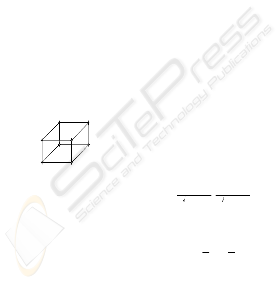
points, lines and surfaces correspondingly. As an
example, let’s consider a cube as shown in Figure 1.
3D coordinates of the points a, b, c, d, e, f, g and h
are defined for a wireframe model representation.
Next, the lines are expressed by its beginning and
the ending points as line ab, ef, bd, etc. Finally, the
surfaces are defined as abcd, acge, etc.
Figure 1: 3D model of a cube.
Understanding of the 3D geometry of the object
is necessary since the 2D view will be considered.
Any plane surface in 3D can be expressed as
following (Hearn and Baker, 1997):
Ax + By + Cz + D = 0 (1)
where (x,y,z) is any point on the plane and the
coefficients A, B, C and D are constants describing
the spatial properties of the plane. If three successive
polygon vertices (x
1
, y
1
, z
1
), (x
2
, y
2
, z
2
) and (x
3
, y
3,
z
3
)
are selected A, B, C and D values can be obtained as
following (Hearn and Baker, 1997):
A = y
1
(z
2
-z
3
) + y
2
(z
3
-z
1
) + y
3
(z
1
-z
2
)
(2)
B = z
1
(x
2
-x
3
) + z
2
(x
3
-x
1
) +z
3
(x
1
-x
2
)
(3)
C = x
1
(y
2
-y
3
) + x
2
(y
3
-y
1
) + x
3
(y
1
-y
2
)
(4)
D = –x
1
( y
2
z
3
- y
3
z
2
) – x
2
( y
3
z
1
- y
1
z
3
)
– x
3
( y
1
z
2
- y
2
z
1
)
(5)
2.2 2D Image Construction
Camera model is the main issue to discuss during the
2D image construction process. Because 3D world
coordinates are transformed into the image
coordinates according to the camera model. In this
paper, the perspective camera model is employed
which is applicable to CCD cameras, IIR systems,
X-ray images and etc. A point in the world is
transformed into pixel coordinates after three steps
using perspective camera model which is described
in Zisserman and Hartley, 2003.
First of all, a point
[]
T
zyx
NNNN =
in the
world coordinate frame (WCF) is related to the
camera coordinate frame (CCF) as:
[
]
)( TNRZYXp
c
w
T
cccc
−==
(6)
where
[
]
T
zyx
TTTT =
is the camera position
expressed in the WCF and
c
w
R
is the rotation matrix
relating the two coordinate frames. Recall that point
c
p
satisfies the plane equation as following:
0=+
+
+
DCZBYAX
ccc
(7)
For the second step,
c
p
is expressed in the image
coordinates by using “similar triangles”, a point in
the CCF is transformed to the image coordinate
frame (ICF) as:
[]
T
c
c
c
c
T
i
Z
Y
f
Z
X
fvup
⎥
⎦
⎤
⎢
⎣
⎡
==
(8)
where
f
is the effective focal length.
i
p
is also
affected by the distortion coefficient of the lens and
becomes:
[]
T
T
ddd
vu
v
vu
u
vup
⎥
⎥
⎦
⎤
⎢
⎢
⎣
⎡
+−++−+
==
)(411
2
)(411
2
2222
κκ
(9)
where
κ
is the distortion coefficient of the total lens
system. Finally,
d
p
is expressed in terms of pixel
coordinates by taking pixel size and image centre
into account as:
[]
T
y
y
d
x
x
d
T
pix
C
S
v
C
S
u
yxp
⎥
⎥
⎦
⎤
⎢
⎢
⎣
⎡
++==
(10)
Therefore, camera coordinates of a point is
projected into the image coordinates by using the
camera calibration parameters. Method for finding
the camera calibration parameters is out of scope of
this study. The parameters are assumed to be known
precisely. Camera model block diagram is shown in
Fig. 2.
b
c
d
f
h
a
e
g
FAST WIREFRAME-VISIBILITY ALGORITHM
271
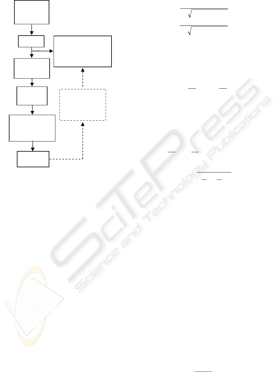
Figure 2: Perspective Camera Model.
2.3 Depth Calculation
Transformation from world frame to the camera
frame results in alignment of the location of the
object with the line of sight direction of the camera.
Thus, visible or invisible parts should be decided in
camera coordinates. At the same time, surface
coefficients A, B, C and D in equation (1) should be
calculated in camera coordinate frame by using the
equations (2), (3), (4) and (5). Since the camera is
located at the origin of the camera coordinate frame,
z coordinate of any point is nothing but its depth
according to the camera. If any two points having
same x and y coordinates are investigated, visible
point has smaller z value than the invisible point
since it is closer to the camera.
In Figure 2, inverse camera model process is also
shown in dashed lines, which converts the image
pixel coordinates to the camera coordinates.
Consequently, depth is calculated by this inverse
process.
Let’s explain the depth calculation step by step.
First,
pix
p
in equation (10) is known and
d
p
can be
obtained directly from
pix
p
as below:
[]
[]
T
yyxx
T
ddd
CySCxSvup )()( −−==
(11)
From equation (9), distorted image coordinates
are known as:
)(411
2
)(411
2
22
22
vu
v
v
vu
u
u
d
d
+−+
=
+−+
=
κ
κ
(12)
From the relations in equation (12), u and v can be
obtained simply by iteration in which known
d
u
and
d
v
values are used. After that, by considering the
equation (8),
c
X
and
c
Y
are calculated as below:
f
Z
vY
f
Z
uX
c
c
c
c
==
(13)
Thus, we obtain the x and y coordinates of the
camera coordinates. By substituting them into
equation (7), the value of
c
Z
, which is exactly equal
to the depth of the point, is found by using the
equation below:
0)()()( =+++ DZC
f
Z
vB
f
Z
uA
c
cc
(14)
C
f
v
B
f
u
A
D
ZDepth
c
++
−
==
(15)
Therefore, depth calculation is succeeded as in
equation (15) for given x and y pixel coordinates of
the point. Coefficients of the plane to which the
point corresponds in 3D should be known, too.
3 THE ALGORITHM
The visible line detection algorithm introduced in
this paper is based on finding the critical points in
the image. Critical points are the intersection points
of the lines in the image. Critical points are simply
found as calculation of intersection of the lines with
known beginning and ending points, slopes and
constant terms. Remember that any line can be
expressed as:
ii
cxmy
+
=
(16)
where
i
m
is the slope and
i
c
is the constant term of
the line. Parameters
i
m
and
i
c
are calculated by
using the beginning (
b
x
,
b
y
) and the ending (
e
x
,
e
y
)
points of the line as following:
eb
eb
xx
yy
m
−
−
=
(17)
R
w
c
, T
3D World
coordinates
p
oint N
Perspective
projection, f
p
c
: 3D camera
coordinates
( X
c
, Y
c
, Z
c
≡ DEPTH )
AX
c
+BY
c
+CZ
c
+D = 0
Transformation
to pixel
coordinates
DEPTH
CALCULATION
inverse camera
mode
l
Internal
Distortion
p
i
p
d
p
pix
VISAPP 2008 - International Conference on Computer Vision Theory and Applications
272
bb
mxyc −=
or
ee
mxyc −
=
(18)
Critical point calculation starts with finding the
intersection point (
tioner
x
secint
,
tioner
y
secint
) of any two
lines having line parameters
1
m
,
1
c
,
2
m
and
2
c
.
21
1221
secint
mm
cmcm
x
tioner
−
−
=
(19)
21
12
secint
mm
cc
y
tioner
−
−
=
(20)
If the intersection points coordinates
tioner
x
secint
and
tioner
y
secint
are in the range of the lines beginning
and ending points, it is regarded as critical points.
Otherwise, it is not a critical point.
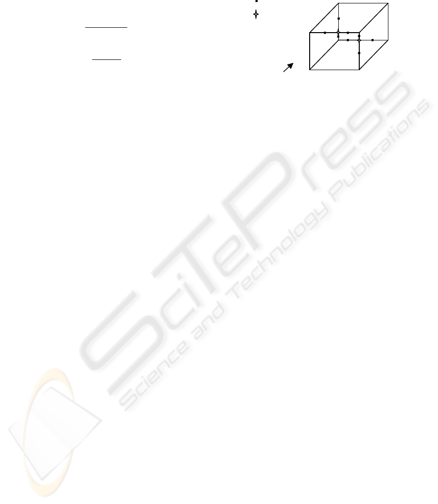
To make the importance and the necessity of the
critical points more clear, let’s work on an example.
In Figure 3, 2D image of a cube is shown without
visible line detection. Camera view side is also
illustrated in the figure. Critical points are marked as
well. It should be noted that the beginning and the
ending points of the lines are not marked even they
are also intersection points. The lines without any
critical points will be investigated after the
investigation of the critical lines.
There is one more important subject one should
notice that any line of a cube is a member of two
surfaces of the cube. This can be shown in Figure 3
since the line fg is a member of the surface afgk and
fgmh. Thus, if we name the surfaces afgk and fgmh
as native surfaces, visibility of the line fg should be
decided according to its native surfaces visibilities.
As observed in Figure 3, point b and d are the
critical points. They are included in the lines ac, fg,
ce, gh which are also called as critical lines.
Therefore, visibility check should be applied to lines
ab, bc, fb, bg, gd, dh, cd, de. It is achieved by taking
the middle points of these lines for two times since
the lines have two native surfaces. Middle points are
also marked in Figure 3. Let’s call these middle
points as m
i
where i is form 1 to 8 for this case. First
of all, the surfaces which include the point m
i
’s
should be listed. This is simply achieved by
checking the coordinates of the point according to
the surface borders coordinates. Note that the native
surfaces will be included in this surface list as well.
Afterwards, at each m
i
the depths of the all surfaces
in the list are calculated as explained in section 2
and are written in the depth matrix. If the minimum
member of the depth matrix is equal to the depth of
the currently selected native surface, the line is
visible and its state should be set to 1. Otherwise it is
hidden and its state should be set to 0. Thus, the
visibilities of the critical lines are decided. One
should recall that this process is done for two times
since a line has two native surfaces for this example.
Figure 3: Critical points of a cube.
When it comes to the visibilities of the normal
lines which do not have any critical points on it, it is
decided in a similar way of the critical lines. In this
case the middle points of the normal lines are taken
and the visibility of that point is investigated just
like critical lines.
To sum up, algorithms steps are presented as
following:
Step 1 Convert the 3D wire-frame from World to
3D camera frame
Step2 Calculate the coefficients (A, B, C and D) of
all the surfaces on the object
Step3 Convert the coordinates from camera to
image frame.
Step4 Calculate the parameters (m and c) of all
lines.
Step5 Calculate the critical points in the image
Step6 Investigate the visibility of the critical lines
one by one by separating the line according to
its critical points.
Step7 Investigate the visibility of the normal lines.
Step8 Plot the visible lines
4 SIMULATION RESULTS
The algorithm is implemented in Matlab. The results
are presented in this section for two experiments.
First, two surfaces with different depths is presented.
In the second experiment, 3D wireframe model is
defined for five prisms. Camera parameters,
rotations and translations are kept same for both of
the experiments.
Figure 4, 5 and 6 are the simulation results for
the first experiment. One triangle and one
parallelogram are defined in 3D wireframe model.
Thus, corner point’s coordinates and the points that
construct the lines and the surfaces are defined. In
a
b
c
d
e
f
g
h
Middle points
Critical points
k
m
Camera
view
FAST WIREFRAME-VISIBILITY ALGORITHM
273
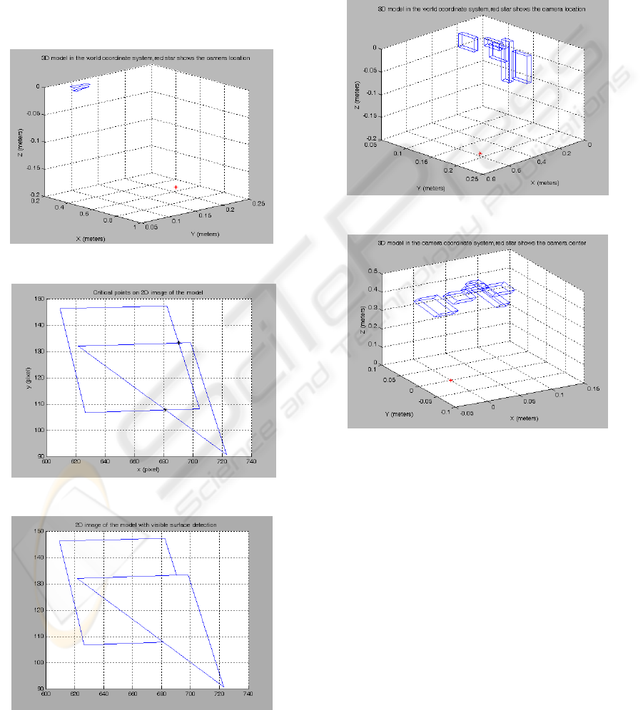
Figure 4, two surfaces are illustrated in the World
coordinate system. Star in the figure shows the
camera location. It is obviously seen in Figure 4 that
the triangle is in front of the parallelogram. After the
transformation from 3D to 2D is applied by using
the camera calibration parameters, Figure 5 is
obtained. Critical points are also marked by stars in
Figure 5. The algorithm runs for 4 critical and 3
normal lines. Figure 6 is the result as expected. 11
pieces of lines are investigated during the algorithm.
Therefore, depth calculation is performed for only
11 times in this experiment.
Figure 4: Two surfaces in the world coordinate frame.
Figure 5: 2D image and the critical points.
Figure 6: 2D image after visible line detection.
For the second experiment, the results are
presented in Figure 7, 8, 9 and 10.
Five prisms are defined having different heights,
widths and lengths. These prisms are shown in
Figure 7 in World coordinate system. Figure 8 is
also put to present the camera coordinate system.
Stars in the figures stand for the camera location. As
shown in Figure 8, camera is at the origin of the
camera coordinate system.
Figure 7: Five prisms in the world coordinate frame.
Figure 8: Five prisms in the camera coordinate frame.
Figure 9 is the 2D image of the prisms without
considering the invisible lines under the camera
parameters. Critical points are also marked in the
figure. Figure 10 is the result of the visible line
detection algorithm. In this experiment, there exist
200 critical points and 60 normal lines. Depth
calculation is done for 321 times. Even though 321
depth calculations seem to be a large number,
duration for the program is shorter than z-buffer or
scan-line method in Matlab. Furthermore, there isn’t
any resolution or memory troubles during the
algorithm.
If the prisms numbers are to be increased, time
for visible line detection will be increased obviously.
However, it would be still faster than the scan-line
or z-buffering methods.
VISAPP 2008 - International Conference on Computer Vision Theory and Applications
274
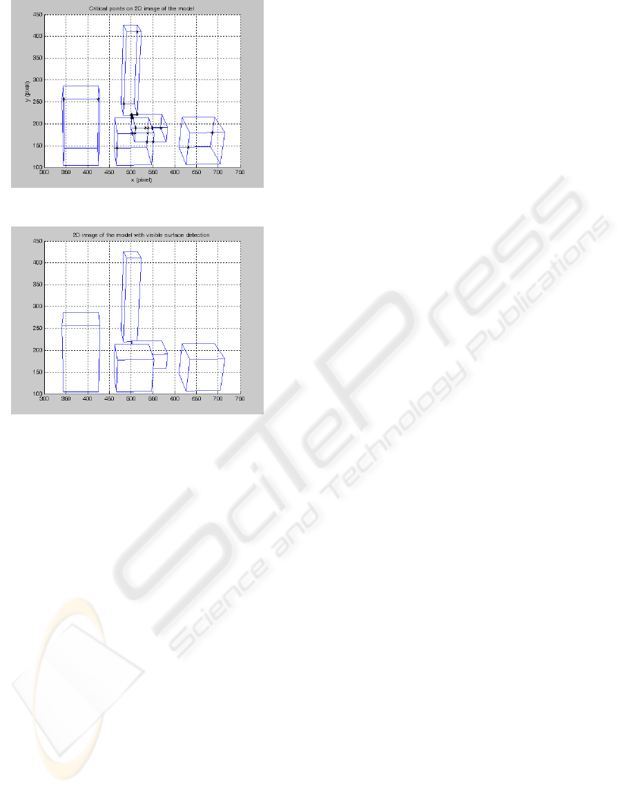
Figure 9: 2D image of prisms and the critical points.
Figure 10: 2D image after visible line detection.
5 CONCLUSIONS
In this paper, a visible line detection algorithm is
introduced for wireframe model. The algorithm is
designed as fast as possible. Such algorithm would
be applicable for air or land vehicles since the rate of
the performance is the most critical term in those
applications.
The algorithm performance should be compared
with the well-known image-space algorithms like z-
buffering and scan-line method in order to conclude
the subject.
The z-Buffer algorithm is one of the most
common hidden-line algorithms to implement in
either software or hardware. The algorithm is an
image-space algorithm. The z-buffer is extension of
the frame buffer idea. Frame buffer is used to store
the attributes (intensity) of each pixel in. The z
buffer is a separate depth buffer, with the same
number of entries as the frame buffer, used to store
the z coordinate or depth of eve- visible pixel in
image-space. Visibility of a pixel is decided by
comparing the z-values of the saved x, y values
(Dong, X., 1999). Conceptually, the algorithm is a
search over x and y and visibility decision is done
pixel by pixel.
When it comes to the scan line algorithms
process the scene in scan line order. Scan line
algorithms operate in image-space. They process the
image one scan line at a time rather than one pixel at
a time. By using area coherence of the polygon, the
processing efficiency is improved over the pixel
oriented method (Dong, X., 1999). However,
resolution of the scan line makes troubles in time
and precision.
The algorithm explained in this paper does not
have any resolution and memory problems. This
algorithm bases on finding the intersection points of
the all lines of the object in 2D image coordinates.
These intersection points are called as critical points
and the lines having them are called as critical lines.
Lines without any critical points are called as normal
lines. Depth calculation is achieved for the separated
critical lines by critical points and the normal lines.
This approach provides much faster process
especially when it is compared with scanning line or
z-buffer methods. The only constraint for this
algorithm is wireframe 3D model representation.
This constraint will not cause any problem in real-
life experiments since any curved shape can be
approximated by defining some lines on that curve.
REFERENCES
Dong, X., 1999, D-Buffer: A new Hidden-Line Algorithm
in Image Space, A master of science thesis submitted
to the Department of Computer Science Memorial
University of Newfoundland, Newfoundland.
Hearn, D., Baker, M.P., 1997, Computer Graphics,
Prentice Hall, Inc., New Jersey, 2
nd
edition.
Zisserman, A., Hartley, R., 2003, Multiple View Geometry
in computer vision, Cambridge University Press,
Cambridge, 2
nd
edition.
FAST WIREFRAME-VISIBILITY ALGORITHM
275
