
CLASSIFIER SELECTION FOR FACE RECOGNITION
ALGORITHM BASED ON ACTIVE SHAPE MODEL
Andrzej Florek and Maciej Król
Institute of Control and Information Engineering, Automatic Control and Robotics Division
Poznań University of Technology, 60-965 Poznań, str. Piotrowo 3A, Poland
Keywords: Face classification, Active Shape Model, Support Vector Machines, Fisher Linear Discriminant Analysis.
Abstract: In this paper, experimental results from the face contour classification tests are shown. The presented
approach is dedicated to a face recognition algorithm based on the Active Shape Model. The results were
obtained from experiments carried out on the set of 2700 images taken from 100 persons. Manually fitted
contours (194 samples for eight components of one face contour) were classified after feature space
decomposition carried out by the Linear Discriminant Analysis or by the Support Vector Machines
algorithms.
1 INTRODUCTION
The presented algorithm for a face classification is
based on the Active Shape Model method (ASM)
(Cootes, 2001), which is a modification of the
Active Contour Model method (Kass, 1988), i.e.
a snake-based approach to extracting face contours
from an image. ASM is based on a shape notation,
which is defined as an ordered set of points and it is
a two-stage algorithm. First, a Point Distribution
Model (PDM) is produced to be used for the
validation of a contour shape. Next, a Local Gray
Level Model (LGLM) is generated for interactive
fitting the contour points to the local image context.
To apply the ASM, an initial contour and its
preliminary location have to be known. This method
is still in progress. Modifications consist of initial
contour choice and the new fitting methods (Zuo,
2004), (Zhao, 2004).
To obtain PDM and LGLM, the desirable
contour localisation on a real image has to be
known. Thus, placing contours onto images chosen
to create a learning set has to be performed. It may
be done manually or semi-automatically. In
presented paper, manually placed contours were
used for testing classifiers. Two methods for the face
contour classification to any class were examined.
The first method was the Nearest Neighbourhood
Classifier (NNC) in reduced Fisher feature subspace
(Linear Discriminant Analysis – LDA) with
Euclidean distance. The second method was the
Support Vector Machines (SVM) with a voting
system or with a criterion based on a maximal
distance from separating classes hyperspaces. A set
of 2700 contours was used to create the learning and
the validation sets and to account classification
accuracy.
2 CONTOURS
The shape in ASM method is represented as an
ordered set of control points placed on contours
describing face elements and it is given by the
following vector
x = ( x
1
, y
1
, x
2
, y
2
,..., x
n
, y
n
)
T
, (1)
Table 1: Face contours.
Contour Number of points
Face outline 41
Mouth outer 28
Mouth inner 28
Right eyelid 20
Left eyelid 20
Right eyebrow 20
Left eyebrow 20
Nose outline 17
TOTAL 194
where x
j
and y
j
are coordinates of shape control
points, expressed in common coordinate frame, for
all shapes in a given set.
276
Florek A. and Król M. (2008).
CLASSIFIER SELECTION FOR FACE RECOGNITION ALGORITHM BASED ON ACTIVE SHAPE MODEL.
In Proceedings of the Third International Conference on Computer Vision Theory and Applications, pages 276-281
DOI: 10.5220/0001077802760281
Copyright
c
SciTePress

In the considered case in the paper, for eight
component face contours of interest, n = 194 such
points have been determined (Fig. 1a and Tab. 1)
and this implies 388 dimensional shape space.
2.1 Extracting and Calculation of
Contours
The stages of applied procedure to obtain normalised
contours are presented in Fig. 1. Images used to
contour extracting are presented in Fig. 2. First, two
landmarks are positioned on the face image, in the
external eye corners. Next, the initial contour
(template) is placed on the image, according to the
landmark positions (Fig. 1a). The landmarks
determine a face pose and an image scale. In the
next step, the contour is manually drawing (fitting)
on place, which seems to the operator as the best
localisation for the contour point positions (Fig. 1b).
Subsequently, the derived contours (Fig. 1c) are
normalised. Scale coefficient results from the
calculated coordinates of eye centres (pupils). This
is connected to applied active shape procedure,
where the initial contour is generally placed
according to expected pupils positions. Pupil
coordinates are calculated from coordinates of
contour samples located in the eyelid corners. X-axis
is determined by pupil coordinates; points (-1,0),
(1,0) are located on right and left pupil, respectively.
The symmetrical of this section determines Y-axis
and the middle of coordinate system. Next, the
contour points are projected on a normalised
coordinate system. The normalised contour has to be
uniformly sampled (manually extracted contours
have nonuniform distances between the adjoining
points). The normalised and uniformly sampled
contours are presented in Fig. 1d. During the
normalisation procedure, points are ordered in
a defined sequence, according to the feature vector
definition (1). In the presented approach, the height
standardizations of face and nose outlines have not
been applied (Fig. 3).
3 EXPERIMENT
In order to select classifiers for ASM method, an
experiment consisting of examining a set of face
images was undertaken. Color images of 2048 ×
1536 pixels were used. For 100 persons (N = 100
classes) the following images were taken:
A – sequence of 30 frames for horizontal head
rotation from the right to the left half-profile;
B – sequence of 20 frames for vertical face rotation
from slightly risen to hanged down head
position;
C – 10 frames for different head position and
limited face mimicry.
The contours were prepared by over a dozen
persons. A person chosen to work on C-frames has
not seen the contours resulting from A and B frames.
The contours were positioned on 11 internal images
from A-frames, on 11 internal images from B-frames
and on 5 images chosen from C-frames (Fig. 2). In
presented experiment 2700 contours were used.
3.1 Set Definitions
The normalised contours were divided into the
following sets:
LS22 – learning set, 2200 contours, 22 for each
class from A- and B-frames;
LS11A – learning set, 1100 contours, 11 for
each class, even subset of LS22;
LS11B – learning set, 1100 contours, 11 for
each class, odd subset of LS22;
LS06 – learning set, 600 contours, 6 for each
class, subset of LS22 with face poses nearest
to en face position;
VS05 – validation set, 500 contours, 5 for each
person from C-frames.
LS11A and LS11B sets were used as learning or
testing sets alternatively.
3.2 Classifiers
Two classifying methods were tested. The first
classifier was Nearest Neighbourhood Classifier in
reduced shape subspace derived from LDA. As
a metric, Euclidean distance to a model of class in
99-dimensional subspace was used. The second
method was taken as the SVM method with kernel
such as Radial Basis Function. The classification of
x sample from testing or learning sets was based on
a voting procedure. In presented approach, a total
number of votes is equal to N (N - 1)/2, where N is
the number of classes. The maximal number of votes
to one class is equal to (N - 1) and in our experiment
it is only 2% of total number of votes. The voting
decision depends only on the sign of discrimination
function for x sample coordinates. In the case of
a pair of “very similar classes”, only one vote from
(N - 1) decisions can decide. In the presented
CLASSIFIER SELECTION FOR FACE RECOGNITION ALGORITHM BASED ON ACTIVE SHAPE MODEL
277
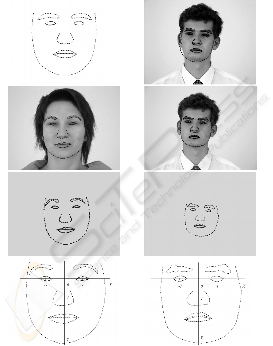
a)
b)
c)
d)
Figure 1: Face contours: a) initial contour and its position on the image, b) images with manually fitted contours,
c) extracted contours, d) normalized contours.
VISAPP 2008 - International Conference on Computer Vision Theory and Applications
278
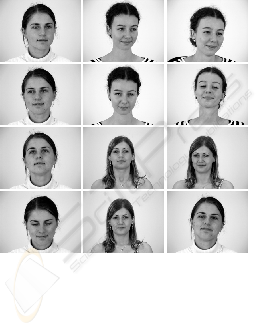
a) b) c)
Figure 2: Images from learning set LS22 (a, b) and validation set VS05 (c): a) boundary frames for sequences symmetrical
to “en face” position, b) boundary frames for nonsymmetrical sequences, c) images from validation set VS05.
example, 70% first succeeding votes for one sample
were: 99, 98 and 97. That is why, one other classifier
for SVM was proposed - the maximal total distance
from all demarcated hyperspaces. Total distance
(margin) td
i
(x) for C
i
class is calculated as
Ν
td
i
(x) = ∑ H
ij
(x) ,
j
= 1
j
≠
i
(2)
where H
ij
(x) is a decision function for the pair of
classes (C
i
, C
j
) and the value is positive if x has been
classified to class C
i
and negative if, it has been
classified to Cj ( H
ij
(x) = 0 is the equation of
boundary hyperspace). The vector x is classified to
the class with maximal td
i
(x) value. The denoting
values of elements in the decision function matrix
between C
i
and Cj classes by decision(i, j), voting
algorithm is, as follow:
CLASSIFIER SELECTION FOR FACE RECOGNITION ALGORITHM BASED ON ACTIVE SHAPE MODEL
279
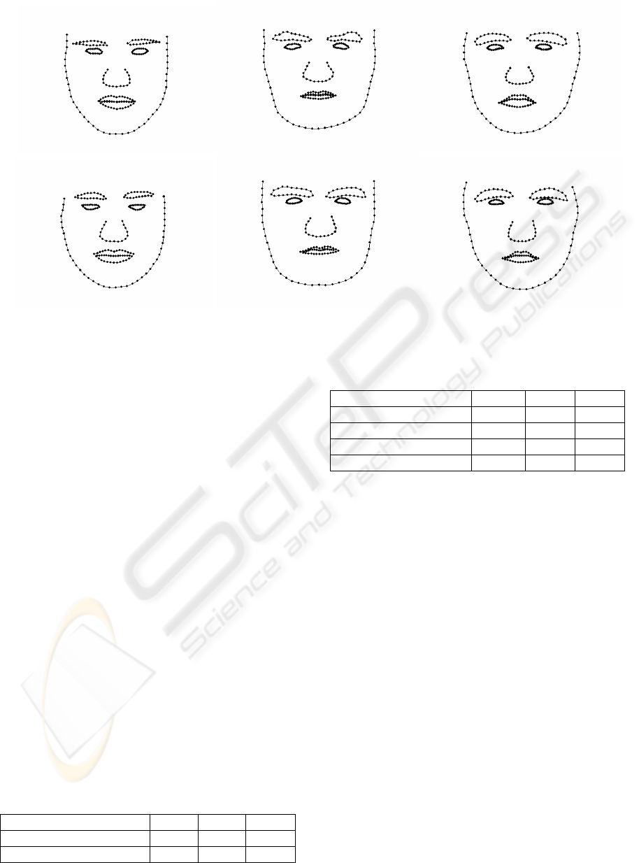
a)
b)
Figure 3: Normalised contours of three people from learning set LS22 (a) and validation set VS05 (b).
IF decision(i,j) > 0
vote(i) += abs(decision(i,j))
vote(j) -= abs(decision(i,j))
ELSE
vote(i) -= abs(decision(i,j))
vote(j) += abs(decision(i,j))
END
The vector x is classified to the class indicated by
the value of
argmax(vote) function.
3.3 Results
As accuracy measure of classifiers, the coefficient
TP/(TP+FP) in percent was chosen, where TP and
FP are True Positive and False Positive numbers of
final classifications. Classification was performed
using 3 methods, named as:
LDA – Fisher Discriminant Analysis and
Euclidean distance in reduced feature space;
SVM-v – SVM and voting system 1-1;
SVM-d – SVM and maximal distance
criterion.
Results are presented in Tab. 2 (for learning and
testing sets) and in Tab. 3 (for validation set).
Table 2: Classification accuracy for learning and testing
sets (in %).
Learning set – testing set LDA SVM-v SVM-d
LS11A – LS11B 99,9 99,3 95,4
LS11B – LS11A 96,5 99,7 97,3
Table 3: Classification accuracy for validation set (in %).
Learning set LDA SVM-v SVM-d
LS22 94,4 78,6 57,0
LS11A 88,2 76,4 58,0
LS11B 68,8 76,6 57,6
LS06 52,8 74,8 53,0
4 SUMMARY
Results in Tab. 2 confirm good propriety of
classifiers, however this is the situation where the
learning and testing sets are nearly regular subsets of
larger learning set LS22. Thus, it is possible to apply
these algorithms to an automatic recognition system
when people want to be recognized. Results in
Tab. 3 are based on tests over the validation set
VS05. Contours belonging to VS05 were manually
posed on others images, not so regular as those in
the learning set LS22 and they were delivered by
other operators. The accuracy in LDA decreases for
smaller learning sets. Lower accuracy for LS11B set
compared with LS11A set possibly results from
different number of images selected from A- and B-
frames. The learning set LS11A has six contours
from A-frames and five contours from B-frames and
LS11B set inversely. The validation set VS05
consisted of frames more similar to A-frames.
Results for SVM methods are rather the same and
whole inferior to LDA. Only for little learning set
VISAPP 2008 - International Conference on Computer Vision Theory and Applications
280

LS06, SVM methods is significant better that LDA
method (more than 40%). The proposed SVM-d
method did not improve classification results. This
may suggest that LDA method is more resistant to
diversity of validation set because the space
transformation function is found in order to
maximize the ratio of between-class variance to
within-class variance. Classifiers based on SVM
transformations, require distinctly representative
learning set. SVM classification is most laborious,
operates in dimensionally higher space and requires
larger voting number than LDA. Presented
experiment shows that even for large but
homogeneous learning set (with relatively small
variance) and various, heterogeneous validation set
(practically normal situation in a visual inspection
system) face classification algorithm based on linear
discriminant analysis seems to be still advisable.
It is desirable to examine influence of other
contour normalisation procedures and to reduplicate
presented experiment, taking into consideration the
contours, automatically calculated by the trained
ASM algorithm. It would be interesting to analyse
how the number of classes N influences the accuracy
of LDA and SVM algorithms.
In presented experiment, the standardisation of
face outline and
nose outline heights has not been
(e.g. to pupils line position). Other normalisation
procedures, application of initial contour determined
by calculated face position (Ge, 2006) and identified
face gestures (de la Torre, 2007) will be verified in
the feature research.
REFERENCES
Cootes, T. and Taylor, C., (2001). Statistical models of
appearance for computer vision, Technical report,
University of Manchester, Wolfson Image Analysis
Unit, Imaging Science and Biomedical Engineering.
Ge, X., Yang, J., Zheng, Z., Li, F., (2006). Multi-view
based face chin contour extraction, Engineering
Applications of Artificial Intelligence, vol.19, pp. 545-
555.
Kass, M., Witkin, A., Terzopoulos, D., (1988). Snakes:
Active contour models, International Journal of
Computer Vision, 1 (4), pp. 321-331.
de la Torre, F., Campoy, J., Coha, J. F., Kanade, T.,
(2007). Simultaneous registration and clustering for
temporal segmentation of facial gestures from video,
Proceedings of the Second International Conference
on Computer Vision Theory and Applications
VISAPP 2007, vol. 2 IU/MTSV, pp. 110-115.
Zhao, M., Li, S. Z., Chen, Ch., Bu, J., (2004). Shape
evaluation for weighted active shape models,
Proceedings of the Asian Conference on Computer
Vision, pp 1074-1079.
Zuo, F. and de With, P. H N., (2004). Fast facial feature
extraction using a deformable shape model with Haar-
wavelet based local texture attributes, Proceedings of
ICIP’04, vol. 3, pp. 1425-1428.
CLASSIFIER SELECTION FOR FACE RECOGNITION ALGORITHM BASED ON ACTIVE SHAPE MODEL
281
