
RECOGNITION OF DYNAMIC VIDEO CONTENTS BASED ON
MOTION TEXTURE STATISTICAL MODELS
∗ Tomas Crivelli, ∗† Bruno Cernuschi-Frias
∗ Faculty of Engineering, University of Buenos Aires, Buenos Aires, Argentina. †CONICET, Argentina
Patrick Bouthemy
IRISA/INRIA, Campus de Beaulieu, 35042 Rennes Cedex, France
Jian-Feng Yao
IRMAR/Univ. of Rennes 1, Campus de Beaulieu, 35042 Rennes Cedex, France
Keywords:
Motion analysis, Markov random fields, image content classification, dynamic textures.
Abstract:
The aim of this work is to model, learn and recognize, dynamic contents in video sequences, displayed mostly
by natural scene elements, such as rivers, smoke, moving foliage, fire, etc. We adopt the mixed-state Markov
random fields modeling recently introduced to represent the so-called motion textures. The approach consists
in describing the spatial distribution of some motion measurements which exhibit values of two types: a
discrete component related to the absence of motion and a continuous part for measurements different from
zero. Based on this, we present a method for recognition and classification of real motion textures using the
generative statistical models that can be learned for each motion texture class. Experiments on sequences from
the DynTex dynamic texture database demonstrate the performance of this novel approach.
1 INTRODUCTION
In the context of visual motion analysis, motion
textures refer to dynamic video contents displayed
mostly by natural scene elements. They are closely
related to temporal or dynamic textures (Doretto et al.,
2003). Different from activities (walking, climbing,
playing) and events (open a door, answer the phone),
temporal textures show some type of stationarity and
homogeneity, both in space and time. Typical exam-
ples can be found in nature scenes: rivers, smoke,
rain, moving foliage, etc.
When analyzing a complex scene, the three types
of dynamic visual information (activities, events and
temporal textures) may be present. However, their
dissimilar nature leads to considering substantially
different approaches for each one in tasks as detec-
tion, segmentation, and recognition.
The aim of this work is to model the apparent mo-
tion contained in dynamic textures, with special inter-
est in dynamic content recognition. Generally speak-
ing, model-based approaches (Doretto et al., 2003;
Saisan et al., 2001; Yuan et al., 2004) have been
mainly dedicated to describe the evolution of inten-
sity over time, while motion-based methods (Fazekas
and Chetverikov, 2005; Lu et al., 2005; Peteri and
Chetverikov, 2005; Vidal and Ravichandran, 2005)
propose the use of motion measurements (mainly
based on optical and normal flow) as input features
for a classification step.
We adopt the mixed-state Markov random fields
(MS-MRF) model introduced in (Bouthemy et al.,
2006), to represent the so-called motion textures. The
approach consists in describing the spatial distribu-
tion of some motion measurements which exhibit val-
ues of two types: a discrete component related to the
absence of motion and a continuous part for real mea-
surements.
Based on this, we present a method for recogni-
tion and classification of real motion textures using
the MS-MRF generative statistical models that can be
learned for each motion texture class. Experiments on
sequences from the DynTex (Peteri et al., 2005) dy-
namic texture database demonstrate the performance
of this novel approach.
283
Crivelli T., Cernuschi-Frias B., Bouthemy P. and Yao J. (2008).
RECOGNITION OF DYNAMIC VIDEO CONTENTS BASED ON MOTION TEXTURE STATISTICAL MODELS.
In Proceedings of the Third International Conference on Computer Vision Theory and Applications, pages 283-289
DOI: 10.5220/0001078102830289
Copyright
c
SciTePress
2 LOCAL MOTION
MEASUREMENTS
In (Fazekas and Chetverikov, 2005), the effectiveness
of normal flow versus complete optical flow measure-
ments, in the context of dynamic texture recognition,
is analyzed. They conclude that for small data sets,
normal flow is an adequate description of temporal
texture dynamics, while complete flow performs bet-
ter when the number of classes grows. However,
they use motion descriptors directly as input features
for the classification step. No underlying statistical
model is proposed.
Our approach consists in defining a statistical
model for motion measurements that allows us to rely
on the representativeness of the model, more than on
the accuracy of the motion measurements. At the
same time, normal flow can be directly computed lo-
cally, avoiding the computational burden associated
to dense flow estimation. Finally, our method is based
on modeling the instantaneous motion maps as spatial
random fields, where the amount of spatial statistical
interaction between motion variables will intervene in
the motion texture recognition.
We consider the normal flow as local motion
measurements. However, in contrast to (Fablet and
Bouthemy, 2003), we do not consider its magnitude
only, but its vectorial expression defined by V
n
(p) =
−
I
t
(p)
k∇
∇
∇I(p)k
∇
∇
∇I(p)
k∇
∇
∇I(p)k
, where p is a location in the image
I. Then, we introduce the following weighted aver-
aging of the normal flow vectors to smooth out noisy
measurements and enforce reliability:
˜
V
n
(p) =
∑
q∈W
V
n
(q) k∇
∇
∇I(q) k
2
max(
∑
q∈W
k∇
∇
∇I(q) k
2
,η
2
)
, (1)
where η
2
is a constant, as in (Fablet and
Bouthemy, 2003), and W is a small window centered
in p. Finally, we consider the following scalar expres-
sion:
v
obs
(p) =
˜
V
n
(p) ·
∇
∇
∇I(p)
k∇
∇
∇I(p) k
, (2)
which projects the smoothed normal motion over the
spatial intensity gradient direction, resulting in v
obs
∈
(−∞,+∞).
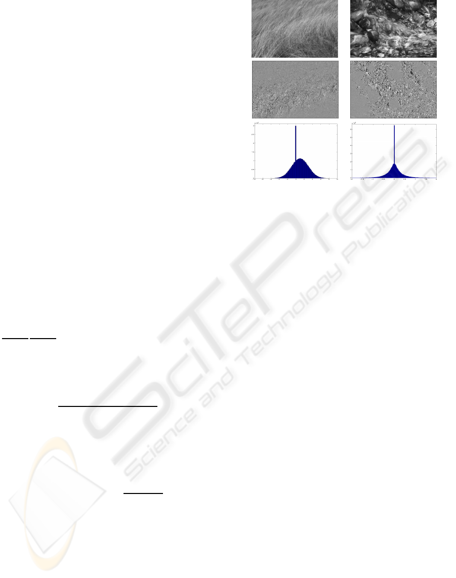
In Fig. 1 we observe the result of applying the pro-
posed motion measurements to two pairs of consecu-
tive images for two different sequences. We observe
in the motion histograms that the statistical distribu-
tion of the motion measurements has two elements: a
discrete component at the null value v
obs
= 0, and a
continuous distribution for the rest of the motion val-
ues. The underlying discrete property of no-motion
a)
b)
c)
Figure 1: a) Images from original sequences (left: straw,
right: water-rocks) obtained from the DynTex texture
database and their corresponding, b) motion textures, and
c) motion histograms.
for a point in the image, is represented as a null ob-
servation, and acts as a symbolic component in the
model. It is not the value by itself that matters, but
the binary property of what is called mobility: the ab-
sence or presence of motion. Thus, the null motion
value in this case, has a peculiar place in the sample
space, and consequently, has to be modeled accord-
ingly.
3 MIXED-STATE MRF MODEL
The key observation made in the previous section
about the statistical properties of motion measure-
ments, settles the necessity for an adequate represen-
tation of the associated random variables. In a first
approach as in (Crivelli et al., 2006), observing the
histograms, the problem can be formulated defining a
probability density for the motion values, that is com-
posed by two terms, i.e.
p(x) = ρδ
0
(x) + (1−ρ) f(x). (3)
where δ
0
(x) is the Dirac impulse function centered
at zero. This density is well-defined and corresponds
to a random variable that has a discrete value with
probability mass concentrated at zero. In fact, it is
easy to observe that P(x = 0) = ρ.
3.1 Measure Theoretic Approach
From a probability theory point of view, it is more
natural to redefine the probability space w.r.t. a new
probability measure, avoiding to deal with a func-
tional or distribution as the Dirac delta, that may com-
VISAPP 2008 - International Conference on Computer Vision Theory and Applications
284

plicate the strict definition of the corresponding den-
sity, allowing also to generalize the case of a discrete
real value (e.g., x = 0) to a generic symbolic value or
abstract label, that may lie on an arbitrary label set.
In this section, we outline the theoretical frame-
work attached to mixed-state random variables. Let
us define M = { r}∪R
∗
where R
∗
= R \{r}, with r
a possible “discrete” value, sometimes called ground
value. A random variable X defined on this space,
called mixed-state variable, is constructed as follows:
with probability ρ ∈(0, 1), set X = r, and with prob-
ability = 1 −ρ, X is continuously distributed in R
∗
.
Hereafter, we will assume that r = 0, without loss of
generality and all the results are inmediately extended
to abstract symbolic values for r. This is the main ad-
vantage of the measure theoretic approach.
Consequently, the distribution function of X can
be expressed as a monotone increasing function with
a “step jump” at X = 0. In order to compute the prob-
ability density function of the mixed-state variable X,
M is equipped with a “mixed” reference measure:
m(dx) = ν
0
(dx) + λ(dx), (4)
where ν
0
is the discrete measure for the value 0 and
λ the Lebesgue measure on R
∗
. Such a measure
has already been used in (Salzenstein and Pieczynski,
1997) for simultaneous fuzzy-hard image segmenta-
tion. Let us define the indicator function of the dis-
crete value 0 as 1
0
(x) and its complementary func-
tion 1
∗
0
(x) = 1
{0}
c
(x) = 1 −1
0
(x). Then, the above
random variable X has the following density function
w.r.t. m(dx):
p(x) = ρ1
0
(x) + (1−ρ)1
∗
0
(x) f(x), (5)
where f(x) is a continuous pdf from an absolutely
continuous distribution w.r.t. λ, defined on R. Equa-
tion (5) corresponds to a mixed-state probability den-
sity.
4 MIXED-STATE SPATIAL
MARKOV MODELS FOR
MOTION TEXTURES
Let X = {x
i
}
i∈1...N
be a motion field or motion texture
obtained as in section 2. We define the neighborhood
N
i
of any image point i, as the 8-point nearest neigh-
bors set, and X
N
i
as the subset of random variables
restricted to N
i
. Then,
N
i
= {i
E
,i
W
,i
N
,i
S
,i
NW
,i
SE
,i
NE
,i
SW
}, (6)
where, for example, i
E
is the east neighbor of i in the
image grid, i
NW
the north-west neighbor, etc.
The following mixed-state conditional model is
considered:
p(x
i
| X
N
i
) = ρ
i
1
0
(x
i
) + (1−ρ
i
)1
∗
0
(x
i
) f (x
i
| X
N
i
,x
i
6= 0)
(7)
where x
i
∈ X is the motion information measurement
at point i ∈ S = {1,..,N} of the image grid and ρ
i
=
P(x
i
= 0 |X
N
i
). Consequently, we have a distribution
consisting of two parts: a discrete component for x
i
=
0 and a continuous one for x
i
6= 0. This model gives
a specific attention to the null value of the random
variable x
i
, which corresponds to the property of no
motion for a point. For the continuous part, f, we
assume a Gaussian density with variance σ
2
i
and mean
m
i
depending on X
N
i
. The motion histograms suggest
the use of this distribution.
In contrast to (Bouthemy et al., 2006), where
a truncated zero-mean Gaussian distribution is as-
sumed, the proposed extension takes into account a
strongest correlation between continuous motion val-
ues, as we will see shortly. This is crucial in our for-
mulation as it allows describing more realistic motion
textures. Then, after some rearrangements, we may
write:
p(x
i
| X
N
i
) = exp
Θ
i
Θ
i
Θ
i
T
(X
N
i
) ·S(x
i
) + logρ
i
(8)
where Θ
i
Θ
i
Θ
i
T
(X
N
i
) ∈ R
d
and S(x
i
) ∈R
d
, with d = 3 for
our case and,
Θ
Θ
Θ
i
(X
N
i
) =
h
log
1−ρ
i
σ
i
√
2πρ
i
−
m
2
i
2σ
2
i
,
1
2σ
2
i
,
m
i
σ
2
i
i
T
(9)
S(x
i
) =
1
∗
0
(x
i
), −x
2
i
, x
i
(10)
As the seminal theorem of Hammersley-Clifford
states, Markov random fields with an everywhere pos-
itive density function, are equivalent to nearest neigh-
bor Gibbs distributions. The joint p.d.f. of the ran-
dom variables that compose the field has the form,
p(X) = exp[Q(X)]/Z, where Q(X) is an energy func-
tion, and Z is called the partition function or normaliz-
ing factor of the distribution. It is a well-known result
in the Markov random fields theory that the energy
Q(X) can be expressed as a sum of potential func-
tions, Q(X) =
∑
C ⊂S
V
C
(X
C
), defined over all subsets
C of the lattice space S (Besag, 1974).
For a one-parameter conditional model (d = 1)
satisfying the assumption that it belongs to the expo-
nential family and that it depends only on cliques that
contain no more than two sites, i.e. auto-models, the
expression for the parameter is known w.r.t. the suffi-
cient statistics S(·) of the neighbors (Besag, 1974). In
the case of multi-parameter auto-models (d > 1), the
result of (Besag, 1974) was extended in (Bouthemy
et al., 2006) and (Cernuschi-Frias, 2007) showing
that:
RECOGNITION OF DYNAMIC VIDEO CONTENTS BASED ON MOTION TEXTURE STATISTICAL MODELS
285

Θ
Θ
Θ
i
(X
N
i
) = α
α
α
i
+
∑
j∈N
i
β
β
β
ij
S(x
j
) (11)
Moreover, they give the expression of the first and
second order potentials of the expansion of the energy
function Q(X):
V
i
(x
i
) = α
α
α
T
i
·S(x
i
) (12)
V
ij
(x
i
,x
j
) = S
T
(x
i
)β
β
β
ij
S(x
j
) (13)
We thus define a mixed-state Markov Random
Field (MS-MRF) auto-model for the motion texture,
where the local conditional probability densities are
mixed-state densities.
4.1 Motion Texture Model Parameters
From equation (11) it is clear that β
β
β
ij
∈ R
3×3
and
α
α
α
i
∈ R
3
. First, we propose that, for the Gaussian
continuous density, f, the conditional mean is given
by,
m
i
(X
N
i
) =
c
i
2b
i
+
∑
j∈N
i
h
ij
2b
i
x
j
(14)
That is, the mean motion value of the continuous part
for a point is a sort of weighted average of the values
of its neighbors. Second, we assume that the variance
is constant for every point, i.e. σ
2
i
(X
N
i
) = σ
2
i
. From
this assumptions, several coefficients of the matrixβ
β
β
ij
are null. Additionally, note that the second order po-
tentials are defined over non-ordered pairs of points
and thus, a symmetry condition arises since V
ij
= V
ji
.
Consequently, from equation (13), β
β
β
ij
= β
β
β
T
ji
. Finally,
we have
β
β
β
ij
=
d
ij
0 0
0 0 0
0 0 h
ij
!
α
α
α
i
= [
a
i
b
i
c
i
]
T
(15)
In general terms, the proposed conditional models
could be defined by a different set of parameters for
each location of the image. This would give rise to
a motion texture model with a number of parame-
ters proportional to the image size. Unfortunately,
such high-dimensional representation of the associ-
ated dynamic information is unfeasible in practice
and does not constitutes a compact description of mo-
tion textures. Moreover, an increasingly number of
frames would be necessary for the estimation pro-
cess. This conspires against a formulation oriented
to efficient content recognition and retrieval. How-
ever, if needed, our framework could deal with spa-
tially non-stationary motion textures. Then, we pro-
pose to use an homogeneous model where α
α
α
i
= α
α
α
and β
β
β
ij
= β
β
β
k
, and k is an index that indicates the
position of the neighbor w.r.t the point, and is inde-
pendent of location i. Moreover, a necessary con-
dition in order to define a stationary spatial process,
is that the parameters related to symmetric neigh-
bors (E-W, N-S, NW-SE, NE-SW) must be the same.
This is a consequence of the symmetry of the po-
tentials. Then, k ∈ {H,V,D,AD}, for the Horizon-
tal, Vertical, Diagonal, and Anti-Diagonal interact-
ing directions. Finally, we have the set of 11 param-
eters which characterizes the motion-texture model,
φ = {a,b, c, d
H
,h
H
,d
V
,h
V
,d
D
,h
D
,d
AD
,h
AD
}.
We now write the expression of the resulting
Gibbs energy for a Gaussian mixed-state Markov ran-
dom field,
Q(X) =
∑
i
a1
∗
(x
i
) −bx
2
i
+ cx
i
+
∑
<i, j>
d
ij
1
∗
(x
i
)1
∗
(x
j
) + h
ij
x
i
x
j
(16)
Here, we distinguish two main parts: a set of terms
related to the interaction between the discrete com-
ponents of the neighbors, and terms related to a con-
tinuous Gaussian Markov random field. Although the
energy is functionally decomposed in two parts, this
does not mean that the two types of values (discrete-
continuous) are independent in the Gibbs field, and
effectively, the estimation of the parameters has to be
done jointly.
4.2 Model-parameter Estimation
In order to estimate the eleven parameters of the
motion-texturemodel from motion measurements, we
adopt the pseudo-likelihood maximization criterion
(Besag, 1974), since the partition function for ex-
act maximum likelihood formulation is in general in-
tractable. Therefore, we search the set of parame-
ters
ˆ
φ that maximizes the function L(φ) =
∏
i∈S
p(x
i
|
X
N
i
,φ). We use a gradient descent technique for the
optimization as the derivatives of L w.r.t φ are known
in closed form.
5 MOTION TEXTURE
RECOGNITION
One of the key aspects of a model oriented to dy-
namic content recognition, as the one proposed here,
is the ability to define a way of computing some sim-
milarity measure between models, in order to embed
it in a decision-theory-based application. In this con-
text, the Kullback-Leibler (KL) divergence is a well-
known distance (more precisely, a pseudo-distance)
VISAPP 2008 - International Conference on Computer Vision Theory and Applications
286

between statistical models. Here we present a result
for computing this quantity between general Gibbs
distributions and obtain an expression for the case of
mixed-state models, that will allow us to classify a set
of real motion textures.
5.1 A Simmilarity Measure Between
Mixed-state Models
The KL divergence from a density p
1
(X) to p
2
(X) is
defined as
KL(p
1
(X) | p
2
(X)) =
Z
Ω
log
p
1
(X)
p
2
(X)
p
1
(X)m(dX), (17)
which is independent of the measure m.
This is not strictly a distance as it is not
symmetric; define then the symmetrized
KL divergence as d
KL
(p
1
(X), p
2
(X)) =
1
2
[KL(p
1
(X) | p
2
(X)) + KL(p
2
(X) | p
1
(X))].
Now, assume that p
1
(X) and p
2
(X) are Markov
random fields, i.e. p
1
(X) = Z
−1
1
expQ
1
(X) and
p
2
(X) = Z
−1
2
expQ
2
(X). Define ∆Q(X) = Q
2
(X) −
Q
1
(X). Then log
p
1
(X)
p
2
(X)
= −∆Q(X) + log
Z
2
Z
1
, and
d
KL
(p
1
(X), p
2
(X)) =
1
2
E
p
2
[∆Q(X)] −E
p
1
[∆Q(X)]
(18)
We observe from this general equation, that we do not
need to have knowledge of the partition functions of
the Gibbs distributions which simplifies enormously
the handling of this expression. Now, let p
1
(X) and
p
2
(X) be two Gaussian MS-MRF. Then,
∆Q(X) =
∑
i
∆αS(x
i
) +
∑
<i, j>
S(x
i
)∆β
ij
S(x
j
) (19)
where ∆α = α
(2)
−α
(1)
and ∆β
ij
= β
(2)
ij
−β
(1)
ij
. From
this definition:
E
p
1
[∆Q(X)] =
∑
i
∆αE
p
1
[S(x
i
)]
+
∑
<i, j>
E
p
1
h
S(x
i
)∆β
ij
S(x
j
)
i
(20)
As we have an homogeneous model, the expectations
in the last equation are equal for each site of the mo-
tion field. The same result applies to E
p
2
[∆Q(X)] and
then it is straightforward to compute equation (18). In
a practical application, the idea is to use the parame-
ters of the two models that we want to compare, to
generate synthetic fields using a Gibbs sampler (Ge-
man and Geman, 1984) from which we can estimate
the involved expectations and finally calculate the di-
vergence.
5.2 Experiments
The recognition performance of mixed-state motion
texture models was tested with real sequences ex-
tracted from the DynTex dynamic texture database
(Peteri et al., 2005). We first took motion textures
where the homogeneity assumption was mostly valid
and divided them in 10 different classes (Figure 2):
steam, straw, traffic, water, candles, shower, flags,
water-rocks, waves, fountain. A total of 30 differ-
ent sequences were considered, and for each one, 5
pairs of consecutive images were selected at frames
1,20,40,60,80, for a total of 150 samples. Each mo-
tion texture class parameter set was learned from a
single pair of images picked from only one of the se-
quences belonging to each type of motion texture. All
sequences were composed by gray scale images with
a resolution of 720x576 pixels, given at a rate of 25
frames per second. In order to reduce computation
time, the original images were filtered and subsam-
pled to a resolution of 180x144 pixels.
Having estimated the reference model parameters
for each of the 10 training samples, we then estimated
φ for each test sample and computed the distance with
each learned parameter vector, as explained in the last
section. The recoginition was based on assigning the
class of motion texture that was closer to the test sam-
ple.
In Table 1 we show the confusion matrix for the
10 motion texture classes. A correct recognition is
considered when both, the test sample and the closest
reference parameter vector, belong to the same class.
A promising overall classification rate of 90.7%
was achieved. As for the confusion matrix, let us
note that it is likely that waves are classified as wa-
ter or water-rocks as they correspond to similar dy-
namic contents, straw is confused with shower, they
have similar vertical orientation, and candles can be
classified as traffic, as both classes show a motion pat-
tern consisting of isolated blobs. The non-symmetry
of the confusion matrix is associated to the nature of
the tested data set, where for some classes, the tested
sequences have a closer resemblance to the training
sample, while for others, there are notorious varia-
tions, that may lead to a misclassification.
Reported experiments for dynamic texture recog-
nition using a model-based approach as the one pre-
sented in (Saisan et al., 2001), have shown a classi-
fication rate of 89.5%, on similar data sets. Their
method is based on computing a subspace distance
between the linear models learned for each class, that
describe the evolution of image intensity over time.
Although the efectiveness of this approach is similar
to ours, the method proposed here has a big advan-
RECOGNITION OF DYNAMIC VIDEO CONTENTS BASED ON MOTION TEXTURE STATISTICAL MODELS
287
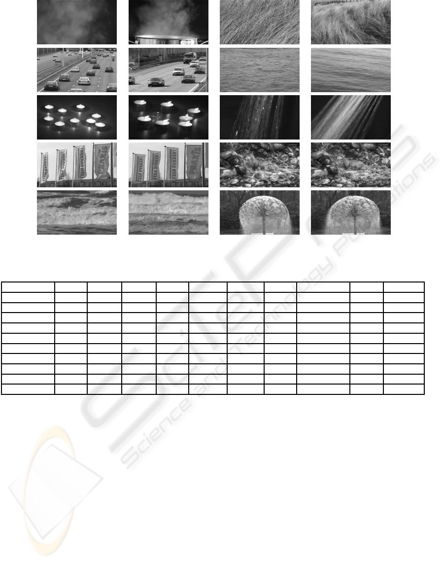
Figure 2: Sample images from the 10 motion texture classes used for the recognition experiments.
Table 1: Motion texture class confusion matrix. Each row indicates how the samples for a class were classified.
steam straw traffic water candles shower flags water-rocks waves fountain
steam 100% - - - - - - - - -
straw - 93.3% - - - 6.7% - - - -
traffic - - 86.7% - - - - 13.3% - -
water - - - 100% - - - - - -
candles - - 13.3% - 73.4% - - 13.3% - -
shower 20% - - - - 80% - - - -
flags - - - - - - 100% - - -
water-rocks - - - - - - - 93.3% - 6.7%
waves - - - 6.7% - - - 13.3% 80% -
fountain - - - - - - - - - 100%
tage, that is, we only need two consecutive frames to
estimate and recognize the mixed-state models, while
in (Saisan et al., 2001) subsequences of 75 frames are
used. This is a consequence of modeling the spatial
structure of motion rather than the time evolution of
the image.
Motion-based methods for dynamic texture clas-
sification (Fazekas and Chetverikov, 2005; Peteri and
Chetverikov, 2005) have shown an improved perfor-
mance with recognition rates of over 95% using in-
variant flow statistics. Although they are the most
accurate reported results for addressing this problem,
they do not provide a general characterization of dy-
namic textures, as model-based approaches do. Con-
sequently, more complex scenarios with combined
problems, as simultaneous detection, segmentation
and recognition of these type of sequences are not di-
rectly addressable. Our framework provides an uni-
fied statistical representation suitable of beeing ap-
plicable to other complex problems, as well (Crivelli
et al., 2006; Bouthemy et al., 2006).
6 CONCLUSIONS
We have presented a novel comprehensive motion
modeling framework for motion texture recognition.
Our approach appropriately handles the mixed-state
nature of motion measurements where the parametric
representation of the statistical models showed quite
satisfactory results on motion texture recognition. In
our method, we do not need to process the whole se-
quence to obtain a reliable estimate of the model in
order to achieve an accurate classification rate. The
approach is entirely valid, with minor modifications,
VISAPP 2008 - International Conference on Computer Vision Theory and Applications
288

for motion texture detection as well. Moreover, the
reference classes can be learned from a single instan-
taneous motion map allowing, eventually, to define an
adaptive scheme for recognition and classification.
Future prospects are based on considering other
dissimilarity measures between statistical models,
combining the classification and detection approach
with existing motion or dynamic texture segmentation
methods and considering the introduction of contex-
tual information through discriminative models, pos-
sibly in the form of Conditional Markov Random
Fields (CMRF).
REFERENCES
Besag, J. (1974). Spatial interaction and the statistical anal-
ysis of lattice systems. Journal of the Royal Statistical
Society. Series B, 36:192–236.
Bouthemy, P., Hardouin, C., Piriou, G., and Yao, J. (2006).
Mixed-state auto-models and motion texture model-
ing. Journal of Mathematical Imaging and Vision,
25:387–402.
Cernuschi-Frias, B. (2007). Mixed-states markov random
fields with symbolic labels and multidimensional real
values. Rapport de Recherche INRIA.
Crivelli, T., Cernuschi, B., Bouthemy, P., and Yao, J. (2006).
Segmentation of motion textures using mixed-state
markov random fields. In Proceedings of SPIE, vol-
ume 6315, 63150J.
Doretto, G., Chiuso, A., Wu, Y., and Soatto, S. (2003).
Dynamic textures. Intl. Journal of Comp. Vision,
51(2):91–109.
Fablet, R. and Bouthemy, P. (2003). Motion recognition
using non-parametric image motion models estimated
from temporal and multiscale co-ocurrence statistics.
IEEE Trans. on Pattern Analysis and Machine Intelli-
gence, 25(12):1619–1624.
Fazekas, S. and Chetverikov, D. (2005). Normal versus
complete flow in dynamic texture recognition: a com-
parative study. In Texture 2005: 4th international
workshop on texture analysis and synthesis. ICCV’05,
Beijing, pages 37–42.
Geman, S. and Geman, D. (1984). Stochastic relaxation,
gibbs distributions, and the bayesian restoration of im-
ages. IEEE Transactions on Pattern Analysis and Ma-
chine Intelligence, 6:721–741.
Lu, Z., Xie, W., Pei, J., and Huang, J. (2005). Dynamic
texture recognition by spatio-temporal multiresolution
histograms. In IEEE Workshop on Motion and Video
Computing (WACV/MOTION), pages 241–246.
Peteri, R. and Chetverikov, D. (2005). Dynamic texture
recognition using normal flow and texture regularity.
In Proc. of IbPRIA, Estoril, pages 223–230.
Peteri, R., Huiskes, M., and Fazekas, S. (2005). Dyn-
tex: A comprehensive database of dynamic textures.
http://www.cwi.nl/projects/dyntex/index.html.
Saisan, P., Doretto, G., Wu, Y., and Soatto, S. (2001).
Dynamic texture recognition. In Proc. of the IEEE
Conf. on Computer Vision and Pattern Recognition.
CVPR’01, Hawaii, pages 58–63.
Salzenstein, F. and Pieczynski, W. (1997). Parameter es-
timation in hidden fuzzy markov random fields and
image segmentation. Graph. Models Image Process.,
59(4):205–220.
Vidal, R. and Ravichandran, A. (2005). Optical flow esti-
mation and segmentation of multiple moving dynamic
textures. In Proc. of CVPR’05, SanDiego, volume 2,
pages 516–521.
Yuan, L., Wen, F., Liu, C., and Shum, H. (2004). Synthesiz-
ing dynamic textures with closed-loop linear dynamic
systems. In Proc. of the 8th European Conf. on Com-
puter Vision, ECCV’04, Prague, volume LNCS 3022,
pages 603–616.
RECOGNITION OF DYNAMIC VIDEO CONTENTS BASED ON MOTION TEXTURE STATISTICAL MODELS
289
