DEPTH PREDICTION AT HOMOGENEOUS IMAGE STRUCTURES
Sinan Kalkan
1
, Florentin W
¨
org
¨
otter
1
and Norbert Kr
¨
uger
2
1
Bernstein Center for Computational Neuroscience, Univ. of G
¨
ottingen, Germany
2
Cognitive Vision Lab, Univ. of Southern Denmark, Denmark
Keywords:
Depth Prediction, 3D Reconstruction, Perceptual Relations.
Abstract:
This paper proposes a voting-based model that predicts depth at weakly-structured image areas from the depth
that is extracted using a feature-based stereo method. We provide results, on both real and artificial scenes,
that show the accuracy and robustness of our approach. Moreover, we compare our method to different dense
stereo algorithms to investigate the effect of texture on performance of the two different approaches. The
results confirm the expectation that dense stereo methods are suited better for textured image areas and our
method for weakly-textured image areas.
1 INTRODUCTION
In this paper, we are interested in prediction of depth
at homogeneous image patches (called monos in this
paper) from the depth of the edges in the scene using a
voting model. We start by creating a representation of
the input stereo image pair in terms of local features
corresponding to edge-like structures and monos (as
introduced in (Kr
¨
uger et al., 2004) and in section 2).
The depth at edge-like features is extracted using a
feature-based stereo method introduced in (Pugeault
and Kr
¨
uger, 2003). This provides a 3D-silhouette
of the scene which however can include strong out-
liers and ambiguous interpretations in particular when
large disparities and low thresholds on matching sim-
ilarities are used (figure 1). The depth of a certain
mono, then, is voted by the 3D edge-like features that
are part of this 3D-silhouette.
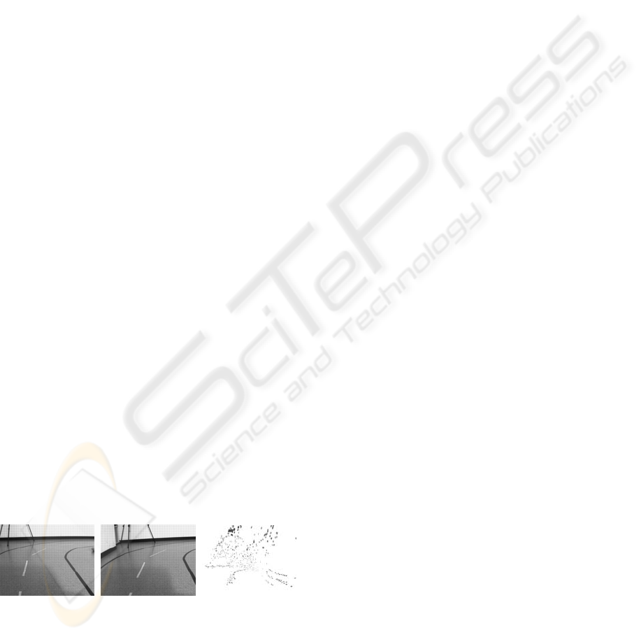
(a) (b) (c)
Figure 1: (a-b)An input stereo pair.(c)Results of a feature-
based stereo algorithm (taken from (Pugeault and Kr
¨
uger,
2003)).
A typical scenario with extracted 3D information
(using stereo) is shown in figure 1. We see that stereo
computation produces strong outliers which prohibit a
direct application of a surface interpolation process as
it is not trivial to differentiate between the outliers and
the reliable stereo information. Moreover, 3D fea-
tures that should be reliable at the edges of the road
turn out not to share a common surface nor a com-
mon 3D line (see figure 1(c)). Therefore, applying a
surface interpolation method on such input data is ex-
pected to lead to an errorneous interpretation of the
scene. In this paper, we will show that our depth pre-
diction method is able to cope with these situations.
We compare our depth prediction method with a
few dense stereo methods (with local as well as global
optimizations) on real and artificial scenes where the
amount of texture can be controlled to see the ef-
fect of texture on the performance of the different ap-
proaches. We show that dense stereo methods are best
suited for textured image areas whereas our method
performs well on homogeneous or weakly-textured
image areas or edges. The results suggest a combi-
nation of both approaches into a single model that
can perform well at both textured and homogeneous
or weakly-textured image areas.
1.1 Related Studies
The work (Grimson, 1982) can be regarded as the
pioneer of surface interpolation studies. In (Grim-
son, 1982), Grimson proposed fitting square Lapla-
cian functionals to surface orientations at existing
3D points utilizing a surface consistency constraint
520
Kalkan S., Wörgötter F. and Krüger N. (2008).
DEPTH PREDICTION AT HOMOGENEOUS IMAGE STRUCTURES.
In Proceedings of the Third International Conference on Computer Vision Theory and Applications, pages 520-527
DOI: 10.5220/0001079005200527
Copyright
c
SciTePress

called ’no news is good news’. The constraint argues
that if two image points do not have a contrast dif-
ference in-between, then they can be assumed to be
on the same 3D surface (see (Kalkan et al., 2006) for
a quantification of this assumption). (Grimson, 1982)
assumes that 3D orientation is available, and the input
3D points are dense enough for second order differen-
tiation.
In (Guy and Medioni, 1994), 3D points with sur-
face orientation are interpolated using a perceptual
constraint called co-surfacity which produces a 3D
association field (which is called the Diabolo field by
the authors) similar to the association field used in 2D
perceptual contour grouping studies. If the points do
not have 3D orientation, they estimate the 3D orienta-
tion first (by fitting a surface model locally) and then
apply the surface interpolation step.
The most relevant studies to our paper are (Hoff
and Ahuja, 1989; Lee et al., 2002). They both argued
that stereo matching and surface interpolation should
not be sequential but rather simultaneous. (Hoff and
Ahuja, 1989) fits local planes to disparity estimates
from zero-crossings of a stereo pair to estimate rough
surface estimates which are then interpolated taking
into account the occlusions, whereas in this paper, we
are concerned with predictions (1) of higher level fea-
tures, (2) using long-range relations and (3) voting
mechanisms. Moreover, as the authors have tested
their approach only on very textured scenes, the appli-
cability of the approach to homogeneous image areas
is not clear. (Lee et al., 2002) employs the following
steps: A dense disparity map is computed, and the
disparities corresponding to inliers, surfaces and sur-
face discontinuities are marked and combined using
tensor voting. The surfaces are then extracted from
the dense disparities using marching cubes approach.
Our work is different from the above mentioned
works in that: Our approach does not assume that the
input stereo points are dense enough to compute their
3D orientation. Instead, our method relies on the 3D
line-orientations of the edge segments which are ex-
tracted using a feature-based stereo algorithm (pro-
posed in (Pugeault and Kr
¨
uger, 2003)). The second
difference is that we employ a voting method which is
different from tensor-voting ((Lee and Medioni, 1998;
Lee et al., 2002)) in that it allows long-range interac-
tions in empty image areas and only in certain direc-
tions in much less computations than tensor-voting, in
order to predict both the depth and the surface orien-
tation.
We would like to distinguish depth prediction
from surface interpolation because surface interpola-
tion assumes that there is already a dense depth map
of the scene available in order to estimate the 3D ori-
entation at points (see, e.g., (Grimson, 1982; Guy and
Medioni, 1994; Lee and Medioni, 1998; Lee et al.,
2002; Terzopoulos, 1988)) whereas our understand-
ing of depth prediction makes use of only 3D line-
orientations at edge-segments which are computed
using a feature-based stereo proposed in (Pugeault
and Kr
¨
uger, 2003).
1.2 Contributions and Outline
Our contributions can be listed as:
• A novel voting-based method for predicting depth
at homogeneous image areas using just the 3D
line orientation at 3D local edge-features.
• Our votes have reliability measures which are
based on the coplanarity statistics of 3D local sur-
face patches provided in (Kalkan et al., 2007).
• Comparison with dense stereo on real and artifi-
cial scenes where we control the amount and the
type of texture to see the effect on performance
of the different approaches. We show that differ-
ent approaches are suited to different kinds of im-
age settings (i.e., textured/weakly-textured), and
the results suggest that a combination of different
approaches is suitable for a model that can per-
form well in all kinds of images.
The paper is organized as follows: In section 2,
we introduce how the images are represented in terms
of local image features. Section 3 describes the 2D
and 3D relations between the local image features that
are utilized in the depth prediction process. Section 4
explains how the depth prediction is performed. In
section 5, the results are presented and discussed. Fi-
nally, section 6 concludes the paper with a summary
and outlook.
2 VISUAL FEATURES
The visual features that we utilize (called primitives in
the rest of the paper) are local, multi-modal features
that were intoduced in (Kr
¨
uger et al., 2004).
An edge-like primitive can be formulated as:
π
e
= (x,θ,ω,(c
l
,c
m
,c
r
)), (1)
where x is the image position of the primitive; θ is
the 2D orientation; ω represents the contrast transi-
tion; and, (c
l
,c
m
,c
r
) is the representation of the color,
corresponding to the left (c
l
), the middle (c
m
) and the
right side (c
r
) of the primitive.
As the underlying structure of a homogeneous im-
age structure is different from that of an edge-like
DEPTH PREDICTION AT HOMOGENEOUS IMAGE STRUCTURES
521

(a)
(b)
(c) (d)
Figure 2: Extracted primitives (b) for the example image in
(a). Magnified edge primitives and edge primitives together
with monos are shown in (c) and (d) respectively.
structure, a different representation is needed for ho-
mogeneous image patches (called monos in this pa-
per):
π
m
= (x,c), (2)
where x is the image position, and c is the color of the
mono. See (Kr
¨
uger et al., 2004) for more information
about these modalities and their extraction. Figure 2
shows extracted primitives for an example scene.
π
e
is a 2D feature which can be used to find corre-
spondences in a stereo framework to create 3D prim-
itives (as introduced in (Pugeault and Kr
¨
uger, 2003))
with the following formulation:
Π
e
= (X,Θ,Ω,(C
l
,C
m
,C
r
)), (3)
where X is the 3D position; Θ is the 3D orienta-
tion; Ω is the phase (i.e., contrast transition); and,
(C
l
,C
m
,C
r
) is the representation of the color, cor-
responding to the left (C
l
), the middle (C
m
) and the
right side (C
r
) of the 3D primitive.
In this paper, we estimate the 3D representation
Π
m
of monos which stereo fails to compute:
Π
m
= (X,n,c), (4)
where X and c are as in equation 2, and n is the orien-
tation (i.e., normal) of the plane that locally represents
the mono.
3 RELATIONS BETWEEN
PRIMITIVES
The sparse and symbolic nature of primitives allows
the following relations to be defined on them. These
relations are used in deciding which features are al-
lowed to make a depth prediction.
3.1 Co–planarity
Two 3D edge primitives Π
e
i
and Π
e
j
are defined to be
co–planar if their orientation vectors lie on the same
plane, i.e.:
cop(Π
e
i
,Π
e
j
) = 1 −|proj
t
j
×v
i j
(t
i
× v
i j
)|, (5)
where v
i j
is the vector (X
i
− X
j
); t
i
and t
j
denote the
vectors defined by the 3D orientations Θ
i
and Θ
j
, re-
spectively; and, proj
u
(a) is the projection of vector a
over vector u.
3.2 Linear Dependence
Two 3D primitives Π
e
i
and Π
e
j
are defined to be lin-
early dependent if the three lines which are defined
by (1) the 3D orientation of Π
e
i
, (2) the 3D orientation
of Π
e
j
and (3) v
i j
are identical. Due to uncertainty in
the 3D reconstruction process, in this work, the lin-
ear dependence of two spatial primitives Π
e
i
and Π
e
j
is
computed using their 2D projections π
e
i
and π
e
j
. We
define the linear dependence of two 2D primitives π
e
i
and π
e
j
as:
lin(π
e
i
,π
e
j
) = |proj
v
i j
t
i
| × |proj
v
i j
t
j
|, (6)
where t
i
and t
j
are the vectors defined by the orienta-
tions θ
i
and θ
j
.
3.3 Co–colority
Two 3D primitives Π
e
i
and Π
e
j
are defined to be co–
color if their parts that face each other have the same
color. In the same way as linear dependence, co–
colority of two spatial primitives Π
e
i
and Π
e
j
is com-
puted using their 2D projections π
e
i
and π
e
j
. We define
the co–colority of two 2D primitives π
e
i
and π
e
j
as:
coc(π
e
i
,π
e
j
) = 1 −d
c
(c
i
,c
j
), (7)
where c
i
and c
j
are the RGB representation of the col-
ors of the parts of the primitives π
e
i
and π
e
j
that face
each other; and, d
c
(c
i
,c
j
) is Euclidean distance be-
tween RGB values of the colors c
i
and c
j
.
Co-colority between an edge primitive π
e
and and
a mono primitive π
m
, and between two monos can be
defined similarly (not provided here).
4 FORMULATION OF THE
MODEL
For the prediction of the depth at monos, we devel-
oped a voting model. Voting models are suitable for
VISAPP 2008 - International Conference on Computer Vision Theory and Applications
522

producing a result from data which includes outliers.
In a voting model, there are a set of voters that state
their opinion about a certain event e. A voting model
combines these votes in a reasonable way to make a
decision about the event e.
In the depth prediction problem, the event e to be
voted about is the depth and the 3D orientation of a
mono π
m
, and the voters are the edge primitives {π
e
i
}
(for i = 1, ..., N
E
) that bound the mono. In this pa-
per, we are interested in the predictions of pairs of
π
e
i
s, which are denoted by P
j
for j = 1,...,N
P
. While
forming a pair P
j
from two edges π
e
i
and π
e
k
from the
set of the bounding edges of a mono π
m
, we have the
following restrictions:
1. π
e
i
and π
e
k
should share the same color with the
mono π
m
(i.e., the following relations should hold:
coc(π
e
i
,π
e
k
) > T
coc
and coc(π
e
i
,π
m
) > T
coc
).
2. The 3D primitives Π
e
i
and Π
e
k
of π
e
i
and π
e
k
should
be on the same plane (i.e., cop(Π
e
i
,Π
e
k
) > T
cop
).
3. π
e
i
and π
e
k
should not be linearly dependent so that
they define a plane (i.e., lin(π
e
i
,π
e
k
) < T
lin
).
The vote v
i
by a pair P
j
can be parametrized by:
v
i
= (X,~n), (8)
where ~n is the normal of the mono π
m
, and X is its
depth.
Each v
i
has an associated reliability or probability
r
i
. They denote how likely the vote is based on the
believes of pair P
i
. It is suggested in (Kalkan et al.,
2007) that the likelihood that a local surface patch is
coplanar with a 3D edge feature decreases with the
distance between them. Accordingly, we define the
reliability r
i
of a vote v
i
as:
r
i
= 1 −
1
min(d(π
m
,π
e
1
),d(π
m
,π
e
2
))
, (9)
where d(.,.) is the Euclidean image distance between
two features.
4.1 Bounding Edges of a Mono
Finding the bounding edges of a mono π
m
requires
making searches in a set of directions d
i
, i = 1,...,N
d
for the edge primitives. In each direction d
i
, start-
ing from a minimum distance R
min
, the search is per-
formed up to a distance of R
max
in discrete steps s
j
,
j = 1,...,N
s
. If an edge primitive π
e
is found in direc-
tion d
i
in the neighborhood Ω of a step s
j
, π
e
is added
to the list of bounding edges and the search continues
with the next direction.
4.2 The Vote of a Pair of Edge
Primitives on a Mono
A pair P
i
of two edge primitives π
e
j
and π
e
k
with two
corresponding 3D edge primitives Π
e
j
and Π
e
k
, which
are co-planar, co-color and linearly independent, de-
fines a plane p with 3D normal n and position X.
The vote v
l
of Π
e
j
and Π
e
k
is computed by the inter-
section of the plane p with the ray l that goes through
the mono, π
m
, and the optical center of the camera.
4.3 Combining the Votes
The votes can be integrated using different ways to
estimate the 3D representation Π
m
of a 2D mono π
m
.
One way is to take the weighted average of the votes.
Weighted averaging is adversely affected by the out-
liers. For this reason, we cluster the votes and do the
averaging inside the best cluster. Let us denote the
clusters by c
i
for i = 1,...,N
c
. Then,
Π
m
= arg max
c
i
#c
i
. (10)
where # is the cardinality of a cluster. The best cluster
can be alternatively chosen to be a cluster which has
the highest reliability. In this paper, we adopted the
definition in equation 10.
Clustering the votes can filter outliers out whereas
it is slow. Moreover, it is not trivial to determine the
number of clusters from the data points that will be
clustered.
In this paper, we implemented (1) a histogram-
based clustering where the number of bins is fixed,
and the best cluster is considered to be the bin with
the most number of elements, and (2) a clustering al-
gorithm where the number of clusters is determined
automatically by making use of a cluster-regularity
measure and maximizing this measure iteratively.
(1) is a simple but fast approach whereas (2)
is considerably slower due to the iterative-clustering
step. Our investigations showed that (1) and (2) pro-
duce similar results (the comparative results are not
provided in this paper). For this reason, we have
adopted (1) as the clustering method for the rest of
the paper.
4.4 Combining the Predictions using
Area Information
3D surfaces project as areas into 2D images. Al-
though one surface may project as many areas in the
2D image, it can be assumed most of the time that the
image points in an image area are part of the same 3D
surface.
DEPTH PREDICTION AT HOMOGENEOUS IMAGE STRUCTURES
523

(a) (b) (c) (d)
Figure 3: (a) The predictions on the surface of the road for the input images shown in figure 1 (predictions are marked with red
boundaries). The predictions are scattered around the plane of the road, and there are wrong predictions due to strong outliers
in the computed stereo. The figure is a snapshot from our 3D displaying software. (b) Segmentation of one of the input images
given in figure 1 into areas using region-growing based on primitives. (c) The surface extracted from the predictions shown
in (a). (d) The predictions from (a) that are corrected using the extracted surface shown in subfigure (c).
Figure 3(a) shows the predictions of a surface.
Due to strong outliers in the stereo computation, depth
predictions are scattered around the surface that they
are supposed to represent. We show that it is possible
to segment the 2D image into areas based on intensity
similarity and combine the predictions in areas to get
a cleaner and more complete surface prediction.
We segment an input image I into areas A
i
, i =
1,..,N
A
using co-colority (see section 3) between
primitives utilizing a simple region-growing method;
the areas are grown until the image boundary or an
edge-like primitive is hit. Figure 3(b) shows the seg-
mentation of one of the images from figure 1.
In this paper, we assume that each A
i
has a corre-
sponding surface S
i
defined as follows:
S
i
(x,y, z) = ax
2
+ by
2
+ cz
2
+ dxy + eyz + fxz + gx +hy + iz = 1.
(11)
Such a surface model allows a wide range of sur-
faces to be represented, including spherical, ellipsoid,
quadratic, hyperbolic, conic, cylinderic and planar
surfaces.
S
i
is estimated from the predictions in A
i
by solv-
ing for the coefficients using a least-squares method.
As there are nine coefficients, such a method requires
at least nine predictions to be available in area A
i
. For
the predictions shown in figure 3(a), the estimated
surface is shown in figure 3(c) using a sparse sam-
pling.
Having an estimated S
i
for an area A
i
makes it pos-
sible to correct the mono predictions using the esti-
mated surface S
i
: Let X
n
be the intersection of the
surface S
i
with the ray that goes through π
m
and the
camera, and n
n
be the surface normal at this point (de-
fined by n
n
= (δS
i
/δ
x
,δS
i
/δ
y
,δS
i
/δ
z
) ). X
n
and n
n
are
respectively the corrected position and the orientation
of mono Π
m
.
Corrected 3D monos for the example scene is
shown in figure 3(d). Comparison with the initial pre-
dictions which are shown in figure 3(a) concludes that
(1) outliers are corrected with the extracted surface
representation, and (2) orientations and positions are
qualitatively better.
Surface information can further be used to remove
the strong outliers in the 3D edge features that are ex-
tracted using stereo.
5 RESULTS
We compared the following: (1) our depth predic-
tion method without surface corrections (DeP); (2) a
phase-based (PB) dense stereo from (Sabatini et al.,
2007); (3) squared sum of differences (SSD) as the
matching function with a winner-take-all approach;
(4) absolute differences as the matching function with
a scanline optimization (SO); and, (5) absolute dif-
ferences with a dynamic programming optimization
(DP). See (Brown et al., 2003) for information about
(3)-(5).
Dense stereo methods (3)-(5) are taken from
(Scharstein and Szeliski, 2001), and their parameters
are adjusted for a good performance as suggested in
(Scharstein and Szeliski, 2001). SO and DP involve a
global optimization step which is expected to improve
results and perform better compared to winner-take-
all approaches. As for PB, the reliability threshold
was set to 0 for better comparabability. The images
which the dense stereo algorithms are applied to were
rectified and downsampled (if needed).
The results of our model as well as DP and PB
(with two different thresholds) is shown in figure 4
for a real scene which includes occlusion and tex-
ture. We see that our method is able to provide com-
parable performance to dense stereo algorithms. Al-
though our algorithm performs well on textured sur-
faces, the effect of the wrong predictions from the oc-
cluding edges are visible especially around the traf-
fic sign. Moreover, due to the uncertainity on the
VISAPP 2008 - International Conference on Computer Vision Theory and Applications
524
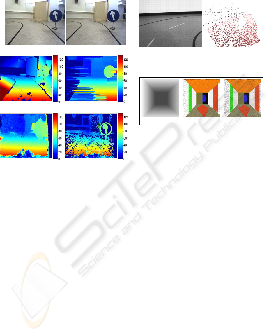
(a) (b)
(c) (d)
(e) (f)
Figure 4: Experiment results on a road scene. (a,b) Input
stereo pair. (c) The predictions of our model as a disparity
map. (d) Disparity map from DP. (e) Disparity map from
PB. (f) Subfigure (e) after a small threshold (0.001).
left edge of the road and as least-squares fitting is af-
fected by the outliers adversely, the surface on the left
is badly reconstructed. Occlusions are a problem for
dense stereo algorithms as well (as seen in e.g., figure
4(e)). DP however can perform better on occluded ar-
eas due to its global optimization; however, DP does
not produce results on the left side of the scene. As
shown in figure 4(f) for PB, using a reliability thresh-
old on the disparity values can get rid of most of the
outliers in figure 4(e), however, lowering the thresh-
old decreases the most of the inliers of the disparity
map.
Another example is shown in figure 5, which
shows that in spite of limited 3D information from
feature-based stereo, our method is able to predict the
surfaces. Figure 5 shows that our method is able to
utilize little information at the right side of the road to
predict the 3D information.
The comparisons are performed on an artificial
scene where the texture could be modified in order
to see the behaviours of the different approaches. The
texture is white noise, and the amount of texture is
controled by the frequency (n ∈ [0,0.2]) of the white-
noise. We tried n up to 0.2 because the images get
Figure 5: Experiment results on a lab road scene. Left: Left
image of the input stereo pair. Right: The predictions of our
model shown in our 3D displaying software.
n=0.1 n=0.2Ground truth
Figure 6: A subset of the textured artificial images that have
been used. Added texture is white noise with a frequency n.
over-textured for bigger values of n. A subset of the
input images are shown in figure 6.
The expectation is to see that dense stereo meth-
ods perform poor on weakly-structured scenes where
our model should make good predictions. When the
amount of texture is increased, dense stereo methods
should perform better, and the predictions made by
our model should degrade because an increase in tex-
ture causes the features to be less reliable and noisy.
For evaluation against a ground truth d
G
, we used
two disparity error measures: Root-Mean-Squares
(RMS) and Bad-Matching-Percentage (BMP). RMS
is the standard measure that has been used in the lit-
erature for evaluating the performance of stereo algo-
rithms (see, e.g., (Scharstein and Szeliski, 2001)):
RMS(S ) =
1
#S
∑
p∈S
|d
C
(p) − d
G
(p)|
2
1/2
, (12)
where S is the set of points with disparity information;
and, d
C
(p) and d
G
(p) are respectively the computed
and the ground truth disparity information at point p.
BMP measure (taken from (Scharstein and
Szeliski, 2001)) is defined as follows:
BMP(S ) =
1
#S
∑
p∈S
(|d
C
(p) − d
G
(p)| > 1), (13)
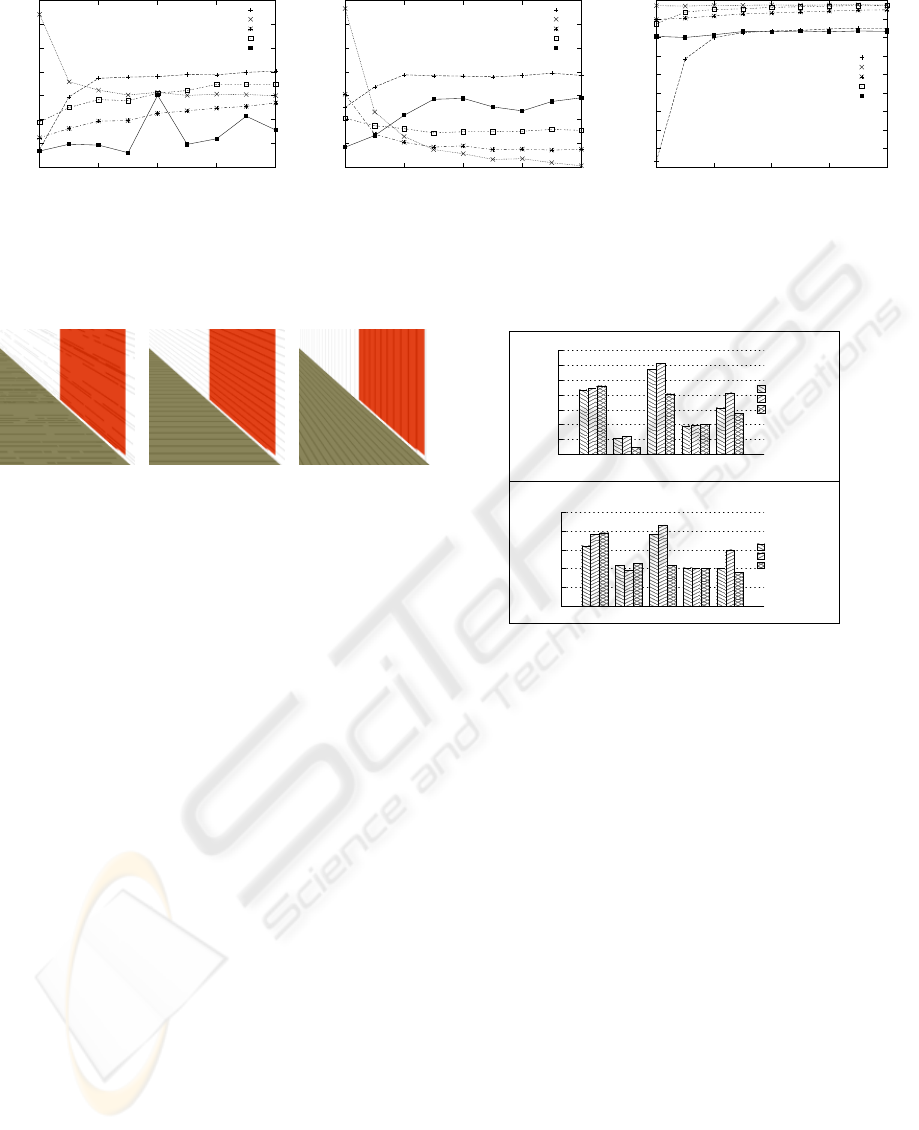
RMS errors in figure 7(a) shows that our method
is more accurate than dense stereo methods. Com-
parison with BMP errors in figure 7(b) suggests RMS
evaluation of dense methods are affected by the out-
liers. In general, we see that when there is no texture,
our method is better than dense methods; the reverse
DEPTH PREDICTION AT HOMOGENEOUS IMAGE STRUCTURES
525
0
5
10
15
20
25
30
35
0 0.05 0.1 0.15 0.2
RMS Error
Amount of texture
PB
SSD
DP
SO
DeP
(a)
20
30
40
50
60
70
80
90
0 0.05 0.1 0.15 0.2
Bad Matching Percentage (%)
Amount of texture
PB
SSD
DP
SO
DeP
(b)
10
20
30
40
50
60
70
80
90
100
0 0.05 0.1 0.15 0.2
Density
Amount of texture
PB
SSD
DP
SO
DeP
(c)
Figure 7: Performance of different algorithms on the artificial scene in figure 6 for different amount of texture using RMS (a),
BMP (b) measures. The densities are shown in (c).
(a) (b) (c)
Figure 8: Weak lines applied on the artificial scene from
figure 6. Due to space constraints, only portions of the im-
ages are provided. (a) Irregular lines. (b) Regular horizontal
lines. (c) Regular vertical lines.
is the case when the image is textured. The density
plot in figure 7(c) confirms that our method can pro-
duce highly dense disparity maps at untextured im-
ages.
We compared the performance of the different ap-
proaches using a different texture on the same artifi-
cial scene from figure 6. The type of texture is weak
lines (see figure 8): regularly sampled vertical and
horizontal lines, and irregularly sampled and sized
lines. The performance of dense stereo methods and
our model are shown in figure 9. Again we observe
that our depth prediction method can provide compa-
rable results to DP, and better results than other ap-
proaches.
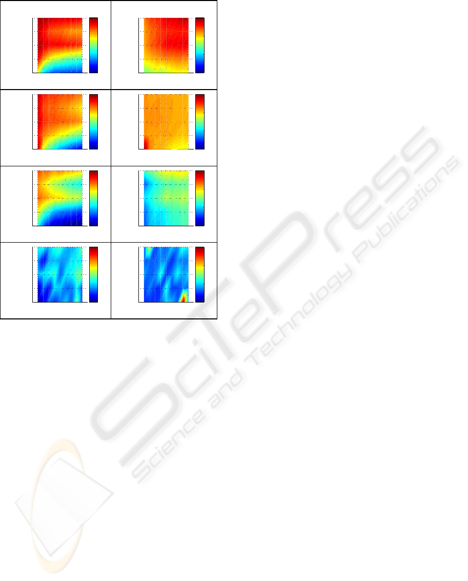
Finally, we compared the performance of the al-
gorithms on noisy images (again using the artificial
scene used above). This comparison is important be-
cause signal to noise ratio at weakly-textured image
areas are higher than textured image areas, for the
same amount of noise. We added white noise with
a frequency between 0 and 0.2 and plotted the per-
formance for different amount of texture (figure 10).
The performance of dense methods are severely af-
fected by noise. Our depth prediction method, on the
other hand, is more robust because edge features are
less sensitive to noise.
Irregular Lines
Horizontal R. Lines
Vertical R. Lines
0
5
10
15
20
25
30
35
SODPSSDDePPB
RMS Error
Irregular Lines
Horizontal R. Lines
Vertical R. Lines
0
20
40
60
80
100
SODPSSDDePPB
Bad Matching Percentage (%)
(b)
(a)
Figure 9: Performance of different algorithms on the arti-
ficial scene in figure 8 for different amount of texture (n)
using RMS (a) and BMP (b) measures.
6 CONCLUSIONS
In this paper, we introduced a voting model that esti-
mates the depth at homogeneous or weakly-textured
image patches from the depth of the bounding edge-
like structures. The depth at edge-like structures is
computed using a feature-based stereo algorithm, and
is used to vote for the depth of a mono, which oth-
erwise is not possible to compute easily due to the
correspondence problem.
The results are compared with different dense
stereo algorithms in order to state that our feature-
based algorithm works well for scenes that dense
stereo algorithms are not suited well. Our aim was
not to claim that our method or dense methods are
better than the other approaches but rather to suggest
a combination of our depth prediction model with a
dense stereo algorithm. Such a combination would
benefit from both approaches and would be able to
work in textured as well as non-textured image areas.
Depth prediction can be regarded as a novel depth
cue which functions at a higher stage than other depth
VISAPP 2008 - International Conference on Computer Vision Theory and Applications
526
0 0.1 0.2
0.01
0.05
0.1
0.15
0.2
Amount of Texture
Amount of Noise
30
40
50
60
70
80
90
0 0.1 0.2
0.01
0.05
0.1
0.15
0.2
Amount of Texture
Amount of Noise
0
10
20
30
0 0.1 0.2
0.01
0.05
0.1
0.15
0.2
Amount of Texture
Amount of Noise
30
40
50
60
70
80
90
0 0.1 0.2
0.01
0.05
0.1
0.15
0.2
Amount of Texture
Amount of Noise
0
10
20
30
0 0.1 0.2
0.01
0.05
0.1
0.15
0.2
Amount of Texture
Amount of Noise
30
40
50
60
70
80
90
0 0.1 0.2
0.01
0.05
0.1
0.15
0.2
Amount of Texture
Amount of Noise
0
10
20
30
0 0.1 0.2
0.01
0.05
0.1
0.15
0.2
Amount of Texture
Amount of Noise
30
40
50
60
70
80
90
0 0.1 0.2
0.01
0.05
0.1
0.15
0.2
Amount of Texture
Amount of Noise
0
10
20
30
DeP DP SSD
BMP RMS
SO
Figure 10: Performance of the different algorithms as a
function of white noise and texture (white noise).
cues and interacts with those cues to fill in missing
depth information. Currently, only the 3D informa-
tion from stereo is made use of; however, any other
depth cue which can provide 3D line orientation at
the edges can be utilized, too.
Depth prediction is along the lines of 3D shape
interpretation from the line drawings of objects. We
are extending our method by integrating the curvature
of the groups in order to make predictions on round
surfaces.
We used a different set of images than for example
the Middleburry database because our method is more
suitable for weakly-textured images, and for surfaces
which are big enough to make predictions at. More-
over, non-availability of the camera parameters for
these images disallows the application of our depth
prediction method, which requires 3D reconstruction
at the edges in order to be able to make depth predic-
tions.
ACKNOWLEDGEMENTS
This work is supported by the European PACO-plus
project (IST-FP6-IP-027657).
REFERENCES
Brown, M. Z., Burschka, D., and Hager, G. D. (2003). Ad-
vances in computational stereo. IEEE Trans. Pattern
Anal. Mach. Intell., 25(8):993–1008.
Grimson, W. E. L. (1982). A Computational Theory of Vi-
sual Surface Interpolation. Royal Society of London
Philosophical Transactions Series B, 298:395–427.
Guy, G. and Medioni, G. (1994). Inference of surfaces from
sparse 3-d points. In ARPA94, pages II:1487–1494.
Hoff, W. A. and Ahuja, N. (1989). Surfaces from stereo:
Integrating feature matching, disparity estimation, and
contour detection. IEEE Trans. Pattern Anal. Mach.
Intell., 11(2):121–136.
Kalkan, S., W
¨
org
¨
otter, F., and Kr
¨
uger, N. (2006). Statistical
analysis of local 3d structure in 2d images. CVPR,
pages 1114–1121.
Kalkan, S., W
¨
org
¨
otter, F., and Kr
¨
uger, N. (2007). First-
order and second-order statistical analysis of 3d and
2d structure. Network: Computation in Neural Sys-
tems, 18(2):129–160.
Kr
¨
uger, N., Lappe, M., and W
¨
org
¨
otter, F. (2004). Bi-
ologically motivated multi-modal processing of vi-
sual primitives. The Interdisciplinary Journal of Ar-
tificial Intelligence and the Simulation of Behaviour,
1(5):417–428.
Lee, M. S. and Medioni, G. (1998). Inferring segmented
surface description from stereo data. In CVPR.
Lee, M.-S., Medioni, G., and Mordohai, P. (2002). Infer-
ence of segmented overlapping surfaces from binoc-
ular stereo. IEEE Trans. Pattern Anal. Mach. Intell.,
24(6):824–837.
Pugeault, N. and Kr
¨
uger, N. (2003). Multi–modal matching
applied to stereo. Proceedings of the BMVC 2003,
pages 271–280.
Sabatini, S. P., Gastaldi, G., Solari, F., Diaz, J., Ros, E.,
Pauwels, K., Hulle, K. M. M. V., Pugeault, N., and
Kr
¨
uger, N. (2007). Compact and accurate early vision
processing in the harmonic space. VISAPP, Barcelona.
Scharstein, D. and Szeliski, R. (2001). A taxonomy and
evaluation of dense two-frame stereo correspondence
algorithms. Technical Report MSR-TR-2001-81, Mi-
crosoft Research, Microsoft Corporation.
Terzopoulos, D. (1988). The computation of visible-surface
representations. IEEE Trans. Pattern Anal. Mach. In-
tell., 10(4):417–438.
DEPTH PREDICTION AT HOMOGENEOUS IMAGE STRUCTURES
527
