
SELF-CALIBRATION OF CENTRAL CAMERAS BY MINIMIZING
ANGULAR ERROR
Juho Kannala, Sami S. Brandt and Janne Heikkil¨a
Machine Vision Group, University of Oulu, Finland
Keywords:
Camera model, camera calibration, self-calibration.
Abstract:
This paper proposes a generic self-calibration method for central cameras. The method requires two-view
point correspondences and estimates both the internal and external camera parameters by minimizing angular
error. In the minimization, we use a generic camera model which is suitable for central cameras with different
kinds of radial distortion models. The proposed method can be hence applied to a large range of cameras from
narrow-angle to fish-eye lenses and catadioptric cameras. Here the camera parameters are estimated by mini-
mizing the angular error which does not depend on the 3D coordinates of the point correspondences. However,
the error still has several local minima and in order to avoid these we propose a multi-step optimization ap-
proach. This strategy also has the advantage that it can be used together with RANSAC to provide robustness
for false matches. We demonstrate our method in experiments with synthetic and real data.
1 INTRODUCTION
The radial distortion of camera lenses is a significant
problem in the analysis of digital images (Hartley and
Kang, 2005). However, traditionally this problem has
been somewhat ignored in the computer vision litera-
ture where the pinhole camera model is often used as a
standard (Hartley and Zisserman, 2003). The pinhole
model is usable for many narrow-angle lenses but it
is not sufficient for omnidirectional cameras which
may have more than 180
◦
field of view (Miˇcuˇs´ık and
Pajdla, 2006). Nevertheless, most cameras, even the
wide-angle ones, are central which means that the
camera has a single effective viewpoint. In fact, there
are basically two kinds of central cameras: catadiop-
tric cameras contain lenses and mirrors while diop-
tric cameras contain only lenses (Miˇcuˇs´ık and Pajdla,
2006). The image projection in these cameras is usu-
ally radially symmetric so that the distortion is merely
in the radial direction.
Recently, there has been a lot of work about build-
ing models and calibration techniques for generic om-
nidirectional cameras, both central and non-central
ones (e.g. (Geyer and Daniilidis, 2001; Ying and Hu,
2004; Claus and Fitzgibbon, 2005; Hartley and Kang,
2005; Ramalingam et al., 2005; Kannala and Brandt,
2006)). In addition, various self-calibration meth-
ods have been proposed for omnidirectional cameras
(Thirthala and Pollefeys, 2005; Barreto and Dani-
ilidis, 2006; Li and Hartley, 2006; Miˇcuˇs´ık and Pa-
jdla, 2006; Ramalingam et al., 2006; Tardif et al.,
2006). Nevertheless, many of these methods still
use some prior knowledge about the scene, such as
straight lines or coplanar points (Li and Hartley, 2006;
Ramalingam et al., 2006; Tardif et al., 2006), or
about the camera, such as the location of the distor-
tion centre (Thirthala and Pollefeys, 2005; Barreto
and Daniilidis, 2006; Miˇcuˇs´ık and Pajdla, 2006). In
fact, despite the recent progress in omnidirectional vi-
sion, there is still a lack of a generic and robust self-
calibration procedure for central cameras. For ex-
ample, the method proposed in (Miˇcuˇs´ık and Pajdla,
2006) uses differentcamera models for different kinds
of central cameras.
In this paper we propose a new general-purpose
self-calibration approach for central cameras. The
method uses two-view point correspondences and es-
timates the camera parameters by minimizing the an-
gular error. In other words, we use the exact expres-
sion for the angular image reprojection error (Olien-
sis, 2002) and write the self-calibration problem as
an optimization problem where the cost function de-
pends only on the parameters of the camera. Since
this cost function appears to have many local min-
ima we propose a stepwise approach for solving the
optimization problem. The experiments demonstrate
that this approach is promising in practice and self-
calibration is possible when reasonable constraints
28
Kannala J., S. Brandt S. and Heikkilä J. (2008).
SELF-CALIBRATION OF CENTRAL CAMERAS BY MINIMIZING ANGULAR ERROR.
In Proceedings of the Third International Conference on Computer Vision Theory and Applications, pages 28-35
DOI: 10.5220/0001079800280035
Copyright
c
SciTePress
Q
O
x
X
q
l
sinθ
cosθ
(12)
X
Z
r
θ
(a)
0 1
0
1
2
true
(12)
(13)
r
θ
π
2
(i)
(ii)
(iii)
(iv)
(v)
(b)
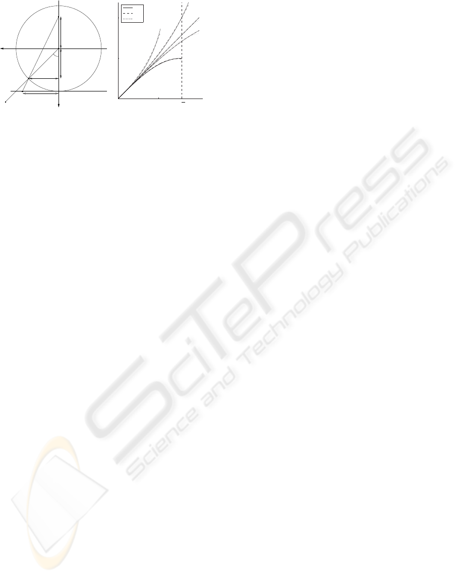
Figure 1: (a) A generic model for a central catadioptric cam-
era (Ying and Hu, 2004). The Z-axis is the optical axis and
the plane Z = 1 is the virtual image plane. The object point
X is mapped to x on the virtual image plane. (b) The pro-
jections (6)-(10) and their approximations with models (12)
and (13).
are provided for the camera parameters. Since the
camera model used in the optimization is generic the
proposed method can be applied to a large range of
central cameras.
2 CENTRAL CAMERA MODELS
In this section we show that a large class of central
cameras can be modelled with a simple model which
contains only one additional degree of freedom com-
pared to the standard pinhole model. This additional
degree of freedom is required for modelling the radial
projection.
2.1 Image Formation in Central
Cameras
A central camera has a single effective viewpoint
which means that the camera measures the intensity
of light passing through a single point in 3D space.
Single-viewpoint catadioptric image formation is well
studied (Baker and Nayar, 1999; Geyer and Dani-
ilidis, 2001) and it has been shown that a central cata-
dioptric projection is equivalent to a two-step map-
ping via the unit sphere (Geyer and Daniilidis, 2001;
Ying and Hu, 2004).
Hence, as described in (Ying and Hu, 2004) and il-
lustrated in Fig. 1(a), a generic model for central cata-
dioptric cameras may be represented as a composed
function
X
G
−→ q
H
−→ x
A
−→ m, (1)
where X = (X,Y,Z)
⊤
is the object point, q is the point
projected on the unit sphere and x = (x,y,1)
⊤
is the
point on the virtual image plane which is mapped
to the observed image point m = (u,v,1)
⊤
by affine
transformation A . The two-step mapping H ◦ G ,
which maps the object point onto the virtual image
plane, is illustrated in Fig. 1(a). There the object point
X is first projected to q on the unit sphere, whose cen-
ter O is the effective viewpoint of the camera. There-
after the point q is perspectively projected to x from
another point Q so that the line through O and Q
is perpendicular to the image plane. The distance
l = |OQ| is a parameter of the catadioptric camera.
The functions G , H and A in (1) have the following
forms
q = G (X) = X/ ||X||
= (cosϕsinθ, sinϕsinθ,cosθ)
⊤
(2)
x = H (q) = (r(θ)cosϕ,r(θ)sinϕ,1)
⊤
(3)
m = A (x) = Kx, (4)
where ϕ and θ are the polar angle coordinates of X, r
is the radial projection function and the affine trans-
formation matrix
K =
f sf u
0
0 γ f v
0
0 0 1
(5)
contains the conventional parameters of a pinhole
camera (Hartley and Zisserman, 2003). The function
r does not depend on ϕ due to radial symmetry and its
precise form as a function of θ is determined by the
parameter l, as illustrated in Fig. 1(a).
The model (1), originally presented for catadiop-
tric cameras (Ying and Hu, 2004), is applicable also
for central dioptric cameras. For example, when Q
coincides with O in Fig. 1(a), the catadioptric projec-
tion model gives the perspective projection
r = tanθ (i. perspective projection), (6)
as a special case. Hence, the pinhole model is in-
cluded in the generalized model (1). However, lenses
with a large field of view, such as fish-eye lenses, are
usually designed to obey one of the following projec-
tion models
r = 2tan(θ/2) (ii. stereographic projection), (7)
r = θ (iii. equidistance projection), (8)
r = 2sin(θ/2) (iv. equisolid angle projection), (9)
r = sin(θ) (v. orthogonal projection), (10)
instead of the perspective projection (Kannala and
Brandt, 2006). In (Kannala and Brandt, 2006) it is
shown that the two-parameter polynomial model
r = k
1
θ+ k
2
θ
3
(11)
provides a reasonable approximation for all the pro-
jections (6)-(10). Below we will show that both
SELF-CALIBRATION OF CENTRAL CAMERAS BY MINIMIZING ANGULAR ERROR
29
the polynomial model and a generalized catadioptric
model provide a basis for a generic one-parameter
projection model so that both of these models allow
reasonable approximation of projections (6)-(10).
2.2 Radial Projection Models
The previous works (Kannala and Brandt, 2006) and
(Ying and Hu, 2004) suggest two different models
for the radial projection function, as discussed above.
The first model is the cubic model
r = θ+ kθ
3
, (12)
and it is obtained from (11) by setting the first-order
coefficient to unity. This does not have any effect on
generality since (3) and (4) indicate that a change in
the scale of r may be absorbed into parameter f in K.
The second model is the catadioptric model based
on (Ying and Hu, 2004) and it has the form
r =
(l + 1)sinθ
l + cosθ
, (13)
which can be deduced from Fig. 1(a), where the corre-
sponding sides of similar triangles must have the same
ratio, i.e.,
r
sinθ
=
l+1
l+cosθ
. In (Ying and Hu, 2004) it
is shown that (13) is a generic model for central cata-
dioptric projections; here we show that it is also a rea-
sonable model for fish-eye lenses. In fact, when l = 0
we have the perspective projection (6), l= 1 gives the
stereographic projection (7) (since tan
θ
2
=
sinθ
1+cosθ
),
and on the limit l → ∞ we obtain the orthogonal pro-
jection (10). Hence, it remains to be shown that (13)
additionally approximates projections (8) and (9).
In Fig. 1(b) we have plotted the projections (6)-
(10) and their least-squares approximations with the
models (12) and (13). The projections were approxi-
mated between 0 and θ
max
so that the interval [0,θ
max
]
was discretized with 0.1
◦
increments. Here the val-
ues of θ
max
were 60
◦
, 110
◦
, 115
◦
, 115
◦
and 90
◦
, re-
spectively, and the model (13) was fitted by using
the Levenberg-Marquardt method. It can be seen that
both models provide a fair approximation for a large
class of radial projections and both of them could be
used in our self-calibration method.
2.3 Backward Models
A central camera can be seen as a ray-based direc-
tional sensor. Hence, when the direction of the in-
coming ray is represented by Φ = (θ,ϕ) the internal
properties of the camera are determined by the for-
ward camera model P which describes the mapping
of rays to the image, m = P (Φ). In our case the for-
ward model P is defined via equations (2)-(4), where
the radial projection function r in (3) is given by (12)
or (13). However, we need to know also the backward
model, Φ = P
−1
(m), and it is computed in two steps:
the inverse of A in (4) is straightforward to compute
and the inversion of r is discussed below.
In the case of model (12), given r and k, the value
of θ is computed by solving a cubic equation. The
roots of a cubic equation are obtained from Cardano’s
formula (R˚ade and Westergren, 1990) and here the
correct root can be chosen based on the sign of k.
In the case of model (13) the mapping from r to θ
is computed as follows. We take squares of both sides
in equation (13) which gives
l
2
r
2
+ 2lr
2
cosθ + r
2
cos
2
θ = (l + 1)
2
sin
2
θ. (14)
Since sin
2
θ = 1− cos
2
θ we get a quadratic equation
in terms of cosθ, and the solution for θ is obtained by
taking the inverse cosine of
cosθ =
−lr
2
±
p
l
2
r
4
− (r
2
+ (l + 1)
2
)(l
2
r
2
− (l + 1)
2
)
(r
2
+ (l+ 1)
2
)
,
(15)
where the +-sign gives the correct solution for pro-
jections such as those in Fig. 1(b).
In summary, based on the discussion above, here
both the forward model P and the backward model
P
−1
can be written as explicit functions of their input
arguments when the values of internal camera param-
eters are given (the five parameters in K and one pa-
rameter in r). This is important considering our self-
calibration method where the backward model will be
needed for evaluating the cost function to be mini-
mized.
3 SELF-CALIBRATION METHOD
In this section we propose a self-calibration method
for central cameras which minimizes the angular two-
image reprojection error over camera parameters. The
method requires two-view point correspondences and
assumes non-zero translation between the views.
3.1 Minimization of Angular Error for
Two Views
Assume that the camera centres of two central cam-
eras are O and O
′
and both cameras observe a point
P. In this case, the epipolar constraint yields
q
′⊤
Eq = 0, (16)
where q and q
′
are the unit direction vectors for
−→
OP and
−−→
O
′
P, represented in the coordinate frames of
VISAPP 2008 - International Conference on Computer Vision Theory and Applications
30

the respective cameras, and E is the essential matrix
(Hartley and Zisserman, 2003). The directions q and
q
′
can be associated with points on the unit sphere and
they correspond to image points m and m
′
via (1).
However, in general, when q and q
′
are obtained
by back-projecting noisy image observations they do
not satisfy (16) exactly which means that the corre-
sponding rays do not intersect. Hence, given E and
q, q
′
, the problem is to find such directions
ˆ
q and
ˆ
q
′
which correspond to intersecting rays and are close
to q and q
′
according to some error criterion. A ge-
ometrically meaningful criterion is the angular error
(Oliensis, 2002) which is the sum of squared sines of
angles between q and
ˆ
q and between q
′
and
ˆ
q
′
, i.e.,
E (q,q
′
,E) = min
ˆ
q,
ˆ
q
′
||
ˆ
q× q||
2
+ ||
ˆ
q
′
× q
′
||
2
(17)
where
ˆ
q
′⊤
E
ˆ
q = 0. This error has an exact closed-form
solution (Oliensis, 2002) and it is
E (q,q
′
,E) =
A
2
−
r
A
2
4
− B, (18)
where
A = q
⊤
E
⊤
Eq+ q
′⊤
EE
⊤
q
′
and
B =
q
′⊤
Eq
2
.
The main idea behind our self-calibration ap-
proach is the following: given a number of two-view
point correspondences we sum the corresponding an-
gular errors (18) and use this sum as a cost function
which is minimized over the camera parameters. In
fact, the essential matrix may be written as a function
of the external camera parameters a
e
, i.e., E = E(a
e
)
(Hartley and Zisserman, 2003). Furthermore, by us-
ing the backward camera model P
−1
the direction
vector q may be represented as a function of the in-
ternal camera parameters, q = q(Φ) = q(P
−1
(m)) =
q(P
−1
(m,a
i
)), where we have explicitly written out
the dependence on the internal parameters a
i
. Hence,
given the point correspondences {m
i
,m
′
i
} we get the
cost function
C(a) =
n
∑
i=1
E (q
i
,q
′
i
,E) =
n
∑
i=1
E
q(P
−1
(m
i
,a
i
)), q(P
−1
(m
′
i
,a
i
)), E(a
e
)
,
(19)
where a = (a
i
,a
e
) denotes the camera parameters.
Minimizing (19) is a nonlinear optimization
problem. Given a good initial guess for a, the solu-
tion can be found by a standard local optimization
algorithm. However, the cost function (19) typically
has several local minima which makes the problem
difficult (Oliensis, 2002). In addition, although there
usually is some prior knowledge about the internal
camera parameters, the initialization of the external
parameters is difficult. Hence, in order to avoid
local minima, we propose a two-phase optimization
approach, where we first perform minimization over
the internal parameters only and use the eight-point
algorithm (Hartley, 1997) to compute the essential
matrix. The outline of the algorithm is as follows.
Generic Algorithm for Self-calibration. Given n ≥
8 correspondences {m
i
,m
′
i
}, the backward camera
model P
−1
, and an initial guess for the internal cam-
era parameters a
i
, estimate the camera parameters
which minimize (19).
(i) Provide a function F which takes a
i
and {m
i
,m
′
i
} as input and gives E as
output: compute correspondences q
i
=
q(P
−1
(m
i
,a
i
)) and q
′
i
= q(P
−1
(m
′
i
,a
i
)) and
use them in the eight-point algorithm (Hart-
ley, 1997).
(ii) Provide a function G which takes a
i
and
{m
i
,m
′
i
} as input and outputs a value of the
error (19): use the function F above to com-
pute E and then simply evaluate (19).
(iii) Minimize G over the internal camera param-
eters.
(iv) Initialize the external camera parameters:
compute E and then retrieve the rotation and
translation parameters (the four solutions are
disambiguated by taking the orientation of
vectors q
i
, q
′
i
into account).
(v) Minimize (19) over all the camera parame-
ters. The initial estimate for the parameters
is provided by steps (iii) and (iv) above.
The self-calibration algorithm is described above
in a very general form. For example, the camera
model and the iterative minimization method are not
fixed there. In the experiments we used the generic
camera models of Section 2 and the iterative mini-
mization in steps (iii) and (v) was performed in Mat-
lab using the function
lsqnonlin
, which is a sub-
space trust region method.
Finally, it should be emphasized that the first four
steps in the algorithm are essential for the perfor-
mance. In fact, in our simulations we experimentally
found that the final estimate is usually less accurate if
the step (iii) is skipped. In addition, the final step (v)
typically gives only slight improvement in the result.
Hence, it seems that our approach, where we first op-
timize over the internal camera parameters, not only
provides a good initialization for the external param-
eters but also allows to avoid local minima.
SELF-CALIBRATION OF CENTRAL CAMERAS BY MINIMIZING ANGULAR ERROR
31

3.2 Constraints on Camera Parameters
In this section, we briefly consider the uniqueness of
the minimum of (19). If the point correspondences
{m
i
,m
′
i
} are exact and consistent with the camera
model P , the minimum value of (19) is 0. How-
ever, it is not self-evident whether this minimum value
is attained at finitely many points in the parameter
space. It is clear that the solution is not unique in
the strict sense since there are four possible solutions
for the motion parameters when E is given up to sign
(Hartley and Zisserman, 2003). In addition, it is well
known that for perspective cameras the constraint of
constant internal parameters is not sufficient for self-
calibration in the two-view case (Hartley and Zisser-
man, 2003). Hence, additional constraints are needed
and here we assume that the values of parameters s
and γ in (5) are known. In particular, the values s= 0
and γ= 1 were used in all our experiments since they
are the correct values for most digital cameras which
have zero skew and square pixels.
3.3 Robustness for Outliers
In practice, the tentative point correspondences
{m
i
,m
′
i
} may contain false matches which can easily
deteriorate the calibration. However, in such cases the
algorithm of Section 3.1 can be used together with the
RANSAC algorithm to provide robustness for false
matches (Hartley and Zisserman, 2003). In detail,
given n correspondences in total, one may randomly
select subsets of p correspondences, p ≪ n, and es-
timate the camera parameters for each subset by the
generic algorithm (the step (v) in the algorithm may
be omitted here for efficiency). Thereafter the esti-
mate which has most inliers according to error (18)
is refined using all the inliers. The value p = 15 was
used in our experiments and the RANSAC algorithm
was implemented following the guidelines in (Hartley
and Zisserman, 2003).
3.4 Three Views
The calibration algorithm described in Section 3.1 ex-
tends straightforwardly to the three-view case. Using
correspondences over three views instead of only two
views increases the stability of the self-calibration. In
addition, the constraints for camera parameters, dis-
cussed in Section 3.2, may be relaxed in the three-
view case if necessary.
The details of the three-viewcalibration procedure
are as follows. Given the point correspondences and
an initial guess for the internal camera parameters,
one may estimate the essential matrix for a pair of
views in the same manner as in the two-view case.
However, now there are three different view pairs and
each pair has its own essential matrix. Our aim is
to minimize the total angular error which is obtained
by summing together the cost functions (19) for each
view pair. The minimization is carried out in a sim-
ilar manner as in the two-view case. First, we mini-
mize the total angular error over the internal camera
parameters (we use the eight point algorithm to com-
pute each essential matrix independently of one an-
other). Thereafter we initialize the external camera
parameters using the estimated essential matrices and
minimize the total angular error over all the camera
parameters.
The three-viewapproachdescribed abovedoes not
require that the point correspondences extend over all
the three views. It is sufficient that there is a set of
two-view correspondences for each view pair. How-
ever, in the case of real data which may contain out-
liers it is most straightforward to use three-view cor-
respondences in the RANSAC framework.
4 EXPERIMENTS
4.1 Synthetic Data
In the first experiment we simulated self-calibration
using randomtwo-viewand three-viewconfigurations
with synthetic data. We used a data set consist-
ing of points uniformly distributed into the volume
[−5,5]
3
\[−2,2]
3
defined by the cubes [−5,5]
3
and
[−2,2]
3
, i.e., there were no points inside the smaller
cube where the cameras were positioned. The first
camera was placed at the origin and the second and
third camera were randomly positioned so that their
distances from the origin were between 1 and 2. In the
three-view case it was additionally required that the
distance between the second and third camera was at
least 1. The orientation of the cameras was such that
at least 40% of the points observed by the first cam-
era were within the field of view of the other cameras.
For each such configuration the points were viewed
by five cameras obeying projections (6)-(10) and the
observed image points were perturbed by a Gaussian
noise with a standard deviation of one pixel. The
true values of the camera parameters were f = 800,
u
0
=500, v
0
=500 for all the five cameras. The maxi-
mum value of the view angle θ was 60 degrees for the
perspective camera, 80 degrees for the orthographic
camera and 90 degrees for the others.
We self-calibrated each of the above five cameras
from varying number of point correspondences us-
VISAPP 2008 - International Conference on Computer Vision Theory and Applications
32
10 30 100 400
0
5
10
15
20
25
number of points
translational error (deg)
catadioptric model
(i)
(ii)
(iii)
(iv)
(v)
10 30 100 400
0
5
10
15
20
number of points
error in rotation axis (deg)
catadioptric model
(i)
(ii)
(iii)
(iv)
(v)
10 30 100 400
0
50
100
150
number of points
error in focal length
catadioptric model
(i)
(ii)
(iii)
(iv)
(v)
10 30 100 400
0
50
100
150
number of points
error in principal point
catadioptric model
(i)
(ii)
(iii)
(iv)
(v)
10 30 100 400
0
10
20
30
40
number of points
RMS reprojection error
catadioptric model
(i)
(ii)
(iii)
(iv)
(v)
10 30 100 400
0
5
10
15
20
25
number of points
translational error (deg)
cubic model
(i)
(ii)
(iii)
(iv)
(v)
10 30 100 400
0
5
10
15
20
number of points
error in rotation axis (deg)
cubic model
(i)
(ii)
(iii)
(iv)
(v)
10 30 100 400
0
50
100
150
number of points
error in focal length
cubic model
(i)
(ii)
(iii)
(iv)
(v)
10 30 100 400
0
50
100
150
number of points
error in principal point
cubic model
(i)
(ii)
(iii)
(iv)
(v)
10 30 100 400
0
10
20
30
40
number of points
RMS reprojection error
cubic model
(i)
(ii)
(iii)
(iv)
(v)
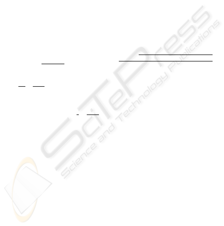
Figure 2: Simulation results in the two-view case with the generalized catadioptric model (top row) and the cubic model
(bottom row). The symbols (i)-(v) refer to five cameras obeying projections (6)-(10) and each point on the plots represents the
median value of 3000 estimates. The first column shows the error in the direction of translation and the second column shows
the error in the rotation axis, both in degrees. The third and fourth column give the errors in the focal length and principal
point in pixels. The last column illustrates the RMS reprojection error.
10 30 100 400
0
5
10
15
number of points
translational error (deg)
catadioptric model
(i)
(ii)
(iii)
(iv)
(v)
10 30 100 400
0
5
10
15
number of points
error in rotation axis (deg)
catadioptric model
(i)
(ii)
(iii)
(iv)
(v)
10 30 100 400
0
20
40
60
80
100
number of points
error in focal length
catadioptric model
(i)
(ii)
(iii)
(iv)
(v)
10 30 100 400
0
50
100
150
number of points
error in principal point
catadioptric model
(i)
(ii)
(iii)
(iv)
(v)
10 30 100 400
0
5
10
15
20
number of points
RMS reprojection error
catadioptric model
(i)
(ii)
(iii)
(iv)
(v)
10 30 100 400
0
5
10
15
number of points
translational error (deg)
cubic model
(i)
(ii)
(iii)
(iv)
(v)
10 30 100 400
0
5
10
15
number of points
error in rotation axis (deg)
cubic model
(i)
(ii)
(iii)
(iv)
(v)
10 30 100 400
0
20
40
60
80
100
number of points
error in focal length
cubic model
(i)
(ii)
(iii)
(iv)
(v)
10 30 100 400
0
50
100
150
number of points
error in principal point
cubic model
(i)
(ii)
(iii)
(iv)
(v)
10 30 100 400
0
5
10
15
20
number of points
RMS reprojection error
cubic model
(i)
(ii)
(iii)
(iv)
(v)
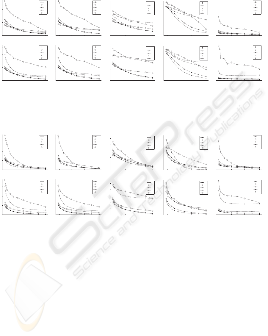
Figure 3: Simulation results in the three-view case. The ordering of the graphs is the same as in Fig. 2. The errors in the
direction of the translation vector and rotation axis are illustrated only for the second view.
ing 3000 distinct two-view and three-view configu-
rations. Since we observed that the step (v) in the
calibration algorithm usually gives only a slight im-
provement in the estimate we skipped it for better effi-
ciency. Hence, the minimization was performed only
over the internal camera parameters which were ran-
domly initialized: the estimate for f was uniformly
distributed on the interval [600,1000] and the esti-
mate for the principal point (u
0
,v
0
) was uniformly
distributed in a 400 × 400 window around the true
value. We used both the cubic (12) and catadioptric
(13) models and the initial values k=0 and l=1 were
used for all the five cameras.
In the two-view case the self-calibration results
are illustrated in Fig. 2 where the graphs illustrate
the errors in the external and internal camera param-
eters. In addition, there is a graph representing the
root-mean-squared(RMS) reprojection error. This er-
ror was calculated by reconstructing each noisy point
correspondence in 3D, reprojecting this point onto the
images and computing the RMS distance between the
reprojected and original points. Each point on the
plots in Fig. 2 represents the median value of the 3000
estimates. It can be seen that the motion estimates are
reasonable and the errors decrease when the number
of points is increased. However, for some cameras
the errors in the internal parameters do not decrease
much. This might indicate that the constraints s= 0
and γ = 1 are not sufficient for all the cameras in the
two-view case. Actually, this is a known fact for a
perspective camera (Hartley and Zisserman, 2003).
Finally, it seems that the catadioptric model works
somewhat better than the cubic model for which the
values of the RMS reprojection error are relatively
high in the case of the perspective camera and orthog-
onal fish-eye camera. However, in general the values
SELF-CALIBRATION OF CENTRAL CAMERAS BY MINIMIZING ANGULAR ERROR
33
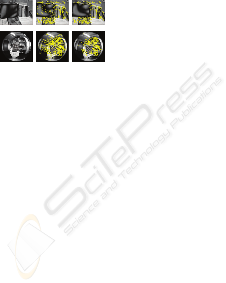
Figure 4: Self-calibration of a conventional (top) and a
fish-eye camera (bottom) using the generalized catadiop-
tric camera model. The tentative correspondences are illus-
trated in the second view (middle), where the flow vectors
indicate several false matches. The last column shows only
the inliers detected during the self-calibration.
of the RMS reprojection error are in the same order
of magnitude as the noise and this indicates that the
optimization has been successful.
In the three-view case the results are illustrated
in Fig. 3. As expected, the errors are smaller than
in the two-view case. Again, the catadioptric model
shows better performance in general. Overall, the
results verify that the proposed approach allows the
self-calibration of generic central cameras given only
a rough initial guess for the internal camera parame-
ters.
4.2 Real Data
In the second experiment we used two cameras, one
was equipped with a conventional lens and the other
with a fish-eye lens. The view pairs taken with these
cameras are shown in Fig. 4. Both cameras were inter-
nally calibrated beforehand and the calibration object,
visible in the images, was used to compute the motion
between the views. Hence, in both cases we know
the correct values of the camera parameters relatively
accurately. The point correspondences between the
view pairs were obtained by matching interest points
using the SIFT descriptor (Lowe, 2004; Mikolajczyk
and Schmid, 2005). In Fig. 4, the putative correspon-
dences are illustrated in the second view, where the
flow vectors indicate several false matches.
For the conventional camera the radial distor-
tion was removed from the images before matching.
Hence, the camera was close to an ideal perspective
camera with the internal parameters f =670, u
0
=328,
v
0
= 252. The self-calibration was performed using
both the cubic and catadioptric models, which were
initialized to the values of k = 0 and l = 1, respec-
tively. The parameter f was initialized to the value
of 500 and the principal point was initially placed at
the image centre. The results of the self-calibration
are shown on the left in Table 1, where the first three
columns illustrate errors in the external parameters
and the next three in the internal parameters. It can be
seen that the error in the focal length is large which
probably reflects the known fact that the constraints
of zero skew and unit aspect ratio are not sufficient
for the full self-calibration of a perspective camera.
Nevertheless, the motion estimate is relatively accu-
rate here too and the 15-point RANSAC procedure
correctly removes the outliers as illustrated in Fig. 4.
In addition, the small median value of the reprojection
error indicates that the optimization has succeeded
and the model fits well to data. Hence, in order to
improve the result more views or constraints on cam-
era parameters would be needed.
Our fish-eye camera was close to the equisolid an-
gle model (9) and the calibrated values for the camera
parameters were f =258, u
0
=506, v
0
=383. The self-
calibration was performed in the same manner as for
the conventional camera; the initial value for f was
500 and the principal point was initially placed at the
image centre. The results are illustrated on the right
in Table 1. It can be seen that the error in the fo-
cal length is much smaller than for the conventional
camera. The result of self-calibration is additionally
illustrated in Fig. 5 where the central region of the
original fish-eye image is warped to follow the per-
spective model using both the initial and estimated
values for the internal camera parameters. The scene
lines, such as the edges of the doors, are straight in
the latter case. This example shows that a rough ini-
tial guess for the camera parameters is sufficient for
self-calibration also in practice.
5 CONCLUSIONS
In this paper, we have proposed a self-calibration
method for central cameras which is based on min-
imizing the two-view angular error over the camera
parameters. The main contributions are the follow-
ing: (1) the generic self-calibration problem was for-
mulated as a small-scale optimization problem where
a single parameter allows to model a wide range of
radial distortions, (2) the optimization problem was
solved using a multi-step approach which allows to
avoid local minima even when only a rough initial
guess is provided for the internal camera parameters.
The experiments demonstrate that our method allows
self-calibration of different types of central cameras
and is sufficiently robust to be applicable for real data.
VISAPP 2008 - International Conference on Computer Vision Theory and Applications
34
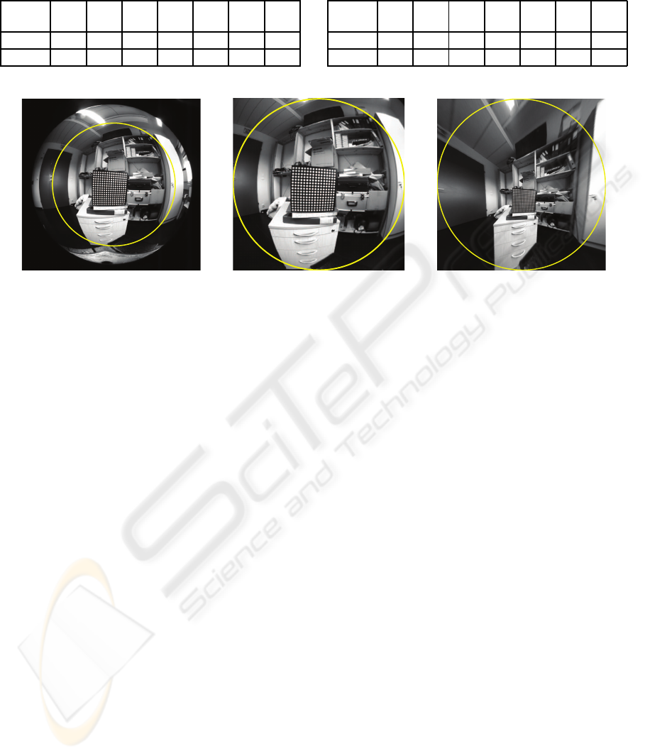
Table 1: The errors in the camera parameters for a conventional and fish-eye camera. Here ∆
a
denotes the error in the rotation
angle, ∆
r
is the error in the direction of the rotation axis and ∆
t
is the translational error, all in degrees. The value ε is the
median of the reprojection error in pixels, i.e., the median distance between the reprojected and observed interest points.
pinhole
∆
a
[deg]
∆
r
[deg]
∆
t
[deg]
∆
f
[pix]
∆
u
0
[pix]
∆
v
0
[pix]
ε
[pix]
(12)
0.40 4.8 0.51 120 4.0 6.5 0.09
(13) 0.59 8.2 0.95 200 1.7 4.9 0.10
fish-eye
∆
a
[deg]
∆
r
[deg]
∆
t
[deg]
∆
f
[pix]
∆
u
0
[pix]
∆
v
0
[pix]
ε
[pix]
(12)
0.11 1.4 20 8.4 10 12 0.26
(13) 0.21 0.43 5.7 0.49 11 14 0.19
Figure 5: Correction of the radial distortion for a fish-eye lens. Left: The original fish-eye image in which the central area is
denoted by the circle. Middle: The area inside the circle is transformed to the perspective model using the initial values for
the internal camera parameters. The transformation is not correct since the scene lines are not straight in the image. Right:
The area inside the circle is corrected using the estimated parameter values. The images of lines are straight.
REFERENCES
Baker, S. and Nayar, S. K. (1999). A theory of single-
viewpoint catadioptric image formation. IJCV, 35(2).
Barreto, J. P. and Daniilidis, K. (2006). Epipolar geometry
of central projection systems using Veronese maps. In
Proc. CVPR.
Claus, D. and Fitzgibbon, A. (2005). A rational func-
tion lens distortion model for general cameras. In
Proc. CVPR.
Geyer, C. and Daniilidis, K. (2001). Catadioptric projective
geometry. IJCV, 45(3).
Hartley, R. and Kang, S. B. (2005). Parameter-free radial
distortion correction with centre of distortion estima-
tion. In Proc. ICCV.
Hartley, R. and Zisserman, A. (2003). Multiple View Geom-
etry in Computer Vision. Cambridge, 2nd edition.
Hartley, R. I. (1997). In defense of the eight-point algo-
rithm. TPAMI, 19(6).
Kannala, J. and Brandt, S. S. (2006). A generic camera
model and calibration method for conventional, wide-
angle, and fish-eye lenses. TPAMI, 28(8).
Li, H. and Hartley, R. (2006). Plane-based calibration and
auto-calibration of a fish-eye camera. In Proc. ACCV.
Lowe, D. (2004). Distinctive image features from scale in-
variant keypoints. IJCV, 60(2).
Miˇcuˇs´ık, B. and Pajdla, T. (2006). Structure from motion
with wide circular field of view cameras. TPAMI,
28(7).
Mikolajczyk, K. and Schmid, C. (2005). A performance
evaluation of local descriptors. TPAMI, 27(10).
Oliensis, J. (2002). Exact two-image structure from motion.
TPAMI, 24(12).
R˚ade, L. and Westergren, B. (1990). Beta, Mathematics
Handbook. Studentlitteratur, Lund, 2nd edition.
Ramalingam, S., Sturm, P. F., and Boyer, E. (2006). A fac-
torization based self-calibration for radially symmet-
ric cameras. In Proc. 3DPVT.
Ramalingam, S., Sturm, P. F., and Lodha, S. K. (2005).
Towards complete generic camera calibration. In
Proc. CVPR.
Tardif, J. P., Sturm, P., and Roy, S. (2006). Self-calibration
of a general radially symmetric distortion model. In
Proc. ECCV.
Thirthala, S. and Pollefeys, M. (2005). Multi-view geome-
try of 1D radial cameras and its application to omni-
directional camera calibration. In Proc. ICCV.
Ying, X. and Hu, Z. (2004). Catadioptric camera calibration
using geometric invariants. TPAMI, 26(10).
SELF-CALIBRATION OF CENTRAL CAMERAS BY MINIMIZING ANGULAR ERROR
35
