PRINCIPLED DETECTION-BY-CLASSIFICATION FROM
MULTIPLE VIEWS
J´erˆome Berclaz
∗
, Franc¸ois Fleuret
∗†
and Pascal Fua
∗
∗
Computer Vision Laboratory, EPFL, Lausanne, Switzerland
†
IDIAP Research Institute, Martigny, Switzerland
Keywords:
People detection, Classification, Bayesian framework.
Abstract:
Machine-learning based classification techniques have been shown to be effective at detecting objects in com-
plex scenes. However, the final results are often obtained from the alarms produced by the classifiers through a
post-processing which typically relies on ad hoc heuristics. Spatially close alarms are assumed to be triggered
by the same target and grouped together.
Here we replace those heuristics by a principled Bayesian approach, which uses knowledge about both the
classifier response model and the scene geometry to combine multiple classification answers. We demonstrate
its effectiveness for multi-view pedestrian detection.
We estimate the marginal probabilities of presence of people at any location in a scene, given the responses
of classifiers evaluated in each view. Our approach naturally takes into account both the occlusions and the
very low metric accuracy of the classifiers due to their invariance to translation and scale. Results show our
method produces one order of magnitude fewer false positives than a method that is representative of typical
state-of-the-art approaches. Moreover, the framework we propose is generic and could be applied to any
detection-by-classification task.
1 INTRODUCTION
Detection in images is often treated as a repeated clas-
sification problem. Given a two-class classifier which
predicts “target present” or “target not present” from
an input signal and a candidate pose (such as location
or scale), detection is achieved by applying it for any
possible pose and collecting the ones associated to
positiveresponses. Such schemes often yield multiple
responses for every single true positive and therefore
require post-processing to refine the outcome.
This step is usually ad hoc and involves grouping
and averaging similar poses corresponding to positive
classifications. Such a procedure is standard for de-
tecting faces (Viola and Jones, 2001; Fleuret and Ge-
man, 2002), cars (Zhao and Nevatia, 2001) and pedes-
trians (Viola et al., 2003; Leibe et al., 2005). Some
people tracking approaches also introduce temporal
consistency to combine the classifier responses in a
stochastic manner (Okuma et al., 2004).
In this paper, we propose a statistically consistent
Bayesian approach for processing answers from re-
peated classification algorithms. As opposed to sim-
ple grouping-and-averaging or non-maximum sup-
pression schemes that are usually applied for this step,
our method takes into account knowledge about both
the classifier response model and the scene geometry,
which yields a more accurate detection with less false
positives.
We demonstrate our approach on the problem of
multi-people detection using several widely spaced
cameras, as illustrated by Fig. 1. In this applica-
tion, a classifier is repeatedly applied to every possi-
ble 3D pose in different camera views, which results
in one map of classifier answers per camera view.
The several maps of classifier answers are then post-
processed and combined by our algorithm to yield the
final detection.
At the heart of our approach is a sophisticated ap-
plication of Bayes’ law. Using a model of the re-
sponses of a classifier given the true occupancy, we
infer a posterior probability on the occupancy given
the classifier responses. We will show that this lets us
combine the multiple and noisy classifier responses in
separate camera views and infer accurate world coor-
dinates for our detections.
Our main contribution is thus a principled ap-
proach for processing detection-by-classification re-
sults and generating a final accurate detection out of
it. When applied to the problem of multi-people de-
tection using several cameras, our approach produces
one order of magnitude fewer false positives than a
375
Berclaz J., Fleuret F. and Fua P. (2008).
PRINCIPLED DETECTION-BY-CLASSIFICATION FROM MULTIPLE VIEWS.
In Proceedings of the Third International Conference on Computer Vision Theory and Applications, pages 375-382
DOI: 10.5220/0001081003750382
Copyright
c
 SciTePress

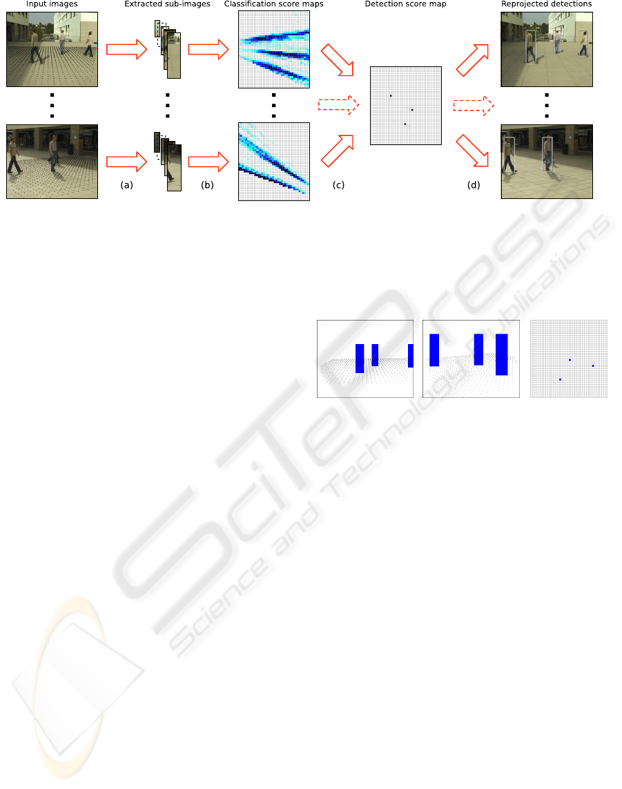
Figure 1: Overview of the detection process. Video sequences are acquired by widely separated and calibrated cameras. The
ground plane of the tracked area is discretized into a finite number of locations, depicted by the black dots in the leftmost
column. (a) We first extract from each image the rectangular sub-images that correspond to the average height of a person at
each of these locations. (b) We apply a classifier trained to recognize pedestrians to each sub-image to estimate probabilities
of occupancy in the ground plane from each view independently. (c) We use the algorithm that is at the core of this paper to
combine the individual classification score maps into a single detection score map. (d) We reproject into the original images
a person-sized rectangle located at local maxima of the probability estimate.
baseline method, that is representative of what is typ-
ically done by state-of-the-art methods. Moreover,
the framework we propose is generic and could be
used with any detection-by-classification application,
whether single or multi view, for which a model of the
classifier response is available.
2 RELATED WORK
We address a problem usually solved by simple ad
hoc solutions. Therefore, even though our frame-
work for processing detection-by-classification re-
sults is generic, we compare it here to pedestrian de-
tection algorithms, which is the application we chose
to demonstrate our method in this paper. Some of the
multi-view pedestrian detection works we reference
below are close in spirit to our framework.
Until recently, most approaches to locating people
in video relied on recursive frame-to-frame pose es-
timation. While effective in some cases, these tech-
niques usually require manual initialization and re-
initialization if the tracking fails. As a result, there
is now increasing interest for techniques that can de-
tect people in individual frames.
A popular approach (Viola et al., 2003; Okuma
et al., 2004; Dalal and Triggs, 2005) is to use
classification-based techniques to decide whether or
not image windows depict a person. Such global
approaches tend to be very occlusion sensitive and
bag-of-features approaches have proved more effec-
tive at detecting pedestrians monocularly in crowded
scenes (Leibe et al., 2005).
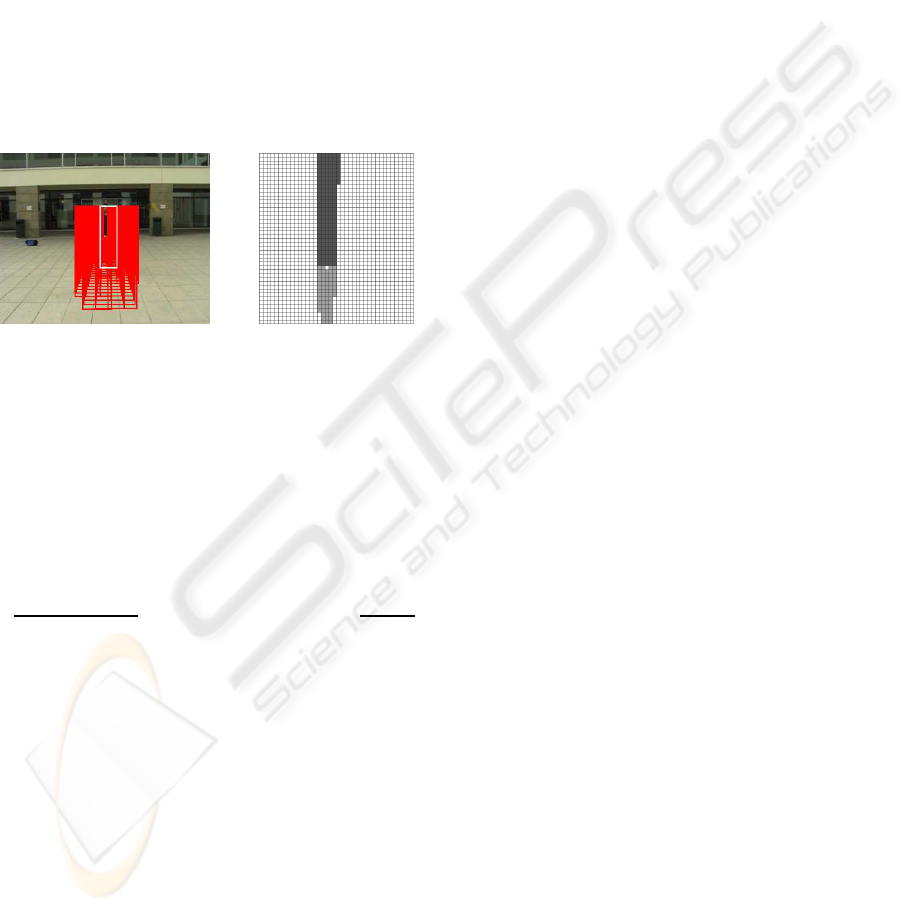
However, with the exceptions of (Khan and Shah,
Figure 2: Correspondence between camera views (left and
center pictures) and top view (right picture) is made through
rectangles computed with ground plane homographies. We
call I
c
(i) the rectangle on camera view c that has the average
shape and position of a pedestrian standing at location i of
the ground plane.
2006; Mittal and Davis, 2003), we are not aware of
many attempts at combining the output of detectors
across views to overcome the problems created by
occlusions in a principled way. In (Khan and Shah,
2006), the algorithm classifies individual pixels as
background or part of a moving object and combines
these results across views by assuming independence
given the presence of a pedestrian at a certain ground
location. Hence, this scheme does not use a generic
pedestrian detector based on a high-levelmodel of sil-
houettes and textures. Neither does it explicitly model
the fact that a detection in one view is influenced
by the presence of distant pedestrians creating occlu-
sions, which, as we will see, can trigger many false
alarms. By contrast, the M
2
Tracker (Mittal and Davis,
2003) explicitly models the relation between mutliple
pedestrians and the image at the pixel level, thus nat-
urally taking occlusions into account. However, this
approach relies on temporal consistency, and since it
is based on a tight integration between the handling
of occlusions and a color-based appearance model, it
can not be generalized to use a generic pedestrian vs.
background classifier.
VISAPP 2008 - International Conference on Computer Vision Theory and Applications
376

Table 1: Notation.
C number of cameras.
G number of locations in the ground plane (≃ 1000).
X
k
boolean random variable standing for the occupancy of
location k on the ground plane.
I
c
input image from camera c.
I
c
(i) rectangular human size sub-window cropped from
camera view c at ground location i.
δ
c
(i, j) horizontal distance between the centers of I
c
(i) and
I
c
( j) on camera view c.
n
c
(i) neighborhood of i on camera c,
{ j 6= i, I
c
( j) ∩ I
c
(i) 6=
/
0}.
T
c
(i) sum of the responses of the binary decision trees at
ground location i in camera view c, thus an integer
value in {0,...,N
T
} where N
T
is the number of deci-
sion trees.
T vector of all the T
c
(i).
Q the product law with the same marginals as the real pos-
terior distribution P( ·|T). Q(X) =
∏
G
i=1
Q(X
i
).
E
Q
expectation under X∼Q. E
Q
(x) =
xQ(x)dx.
q
k
the marginal probability of Q, i.e. Q(X
k
= 1).
k.k area of a sub-image.
In contrast to the approaches described above,
our method relies on classifiers applied on separate
views independently. We explicitly integrate occlu-
sion effects between alarms and quantitative knowl-
edge about the classifier insensitivity to pose change
into a sound Bayesian framework to combine the mul-
tiple classifier answers and yield the final detection.
3 ALGORITHM
We start by giving an overview of our algorithm, be-
fore going into more details in the following subsec-
tions. We use notations summarized in Table 1.
In our setup, an area of interest is filmed by C
widely separated and calibrated cameras. We dis-
cretize the ground plane into a regular grid of G lo-
cations separated by 25cm (Elfes, 1989), and com-
pute homographies that relate the ground plane to its
projections in the camera views. This way, we can de-
termine, for every camera view c and every location
i, the sub-image I
c
(i), which roughly corresponds to
the average size of a person that would be standing
at location i of the ground plane, as shown on Fig. 2.
Our algorithm involves two main steps:
1. For each camera c and ground plane location i,
the algorithm extracts sub-image I
c
(i). Classifiers
based on decision trees are then applied to every
sub-image I
c
(i), as shown on Fig. 3. These clas-
sifiers have been trained at recognizing pedestri-
ans, and their answer on sub-image I
c
(i) can be
interpreted as a rough probability of occupancy
of ground plane location i, given the sub-image.
This first step thus produces as many classifica-
Figure 3: Generation of the classification score maps. Im-
ages (a), (b) and (c) show sub-windows extracted from the
camera view at 3 random locations of the ground plane.
Classifiers are applied to sub-images I
c
(i) corresponding to
every ground plane location i. Images depicting background
(a) produce a low classification score for the correspond-
ing location. Images showing badly centered pedestrian (b)
produce a slightly higher score and images featuring a well
centered pedestrian (c) receive high score.
tion score maps (see third column of Fig. 1) as
there are cameras and is described in §3.1.
2. The several classification score maps, generated
during step 1, are now combined into a final prob-
ability of occupancy map (called hereafter detec-
tion score map), such as the one of the fourth
column of Fig. 1. This represents an estimate
of P(X
i
= 1|I
1
,.. . ,I
C
), the true marginal of the
probabilities of presence at every location, given
the full signal.
We compare two approaches for the second step.
Section §3.2 describes the one, which is representa-
tive of what is usually done by state-of-the-art meth-
ods. We refer to it as the baseline because it combines
the individual classification score maps without tak-
ing into account the interactions between presence of
pedestrian due to occlusion. By constrast, the second
approach takes into account potential occlusions and
knowledge about the classifier behavior and yields a
substantial increase in performance. It is at the core
of our contribution and is discussed in §3.3.
3.1 Classification Score Maps
We introduce the classifier we use for single-view
pedestrian detection and to compute our classification
score maps.
3.1.1 Classifier as a Pedestian Detector
During a learning step, we create a set of decision
trees dedicated to the classification of rectangular im-
ages into two classes: “person” or “background”. The
binary decision trees we use as classifiers are based
on thresholded Haar wavelets operating on grayscale
images (Viola and Jones, 2001). They are trained us-
ing a few thousands of images of different sizes, each
of which represents either a pedestrian correctly cen-
PRINCIPLED DETECTION-BY-CLASSIFICATION FROM MULTIPLE VIEWS
377

Figure 4: The 3 images on the left show the classification
score maps of a scene viewed under three different angles.
The right image represents the corresponding ground truth.
tered in the rectangular frame, or background, which
could be anything else.
More specifically, for every tree, several hundreds
of features of different scales, orientations and as-
pect ratios are generated randomly and applied to our
training set. The one that best separates the two pop-
ulations according to Shanon’s entropy is kept as the
root node and the training set is split and then dropped
into two similarly-constructed sub-nodes (Breiman
et al., 1984). This process is repeated until either the
person and background sets are completely separated
or it reaches the tree maximum depth d = 5. Our clas-
sifier consists of a forest (Breiman, 1996) of N
T
= 21
decision trees built in this manner.
3.1.2 Computing Classification Score Maps
The algorithm iterates through every camera and
ground location, extracts a sub-image corresponding
to the rectangular shape of human size, and takes its
score to be the number of trees classifying the sub-
image as “person” (Fig. 3).
If we see the individual tree responses as many
i.i.d. samples of the response of an ideal classifier,
the classification score in location i is an estimate of
the probability for such a classifier to respond that i is
actually occupied given the subimage at that location.
Hence, it is a good indicator of the actual occupancy.
This produces, for each camera, a map such as the
ones depicted by the third column of Fig. 1 or by the
three left pictures in Fig. 4, which assigns a voting
score to every ground location. As shown on those
figures, detected pedestrians appear as “cone shapes”
in the axis of the camera, on the classification score
maps. This is due to the high tolerance in scale and
limited tolerance in translation of the classifiers, and
hinders precise people location. Hence the need of an
extra step, which combines classification score maps
from different camera views into one accurate detec-
tion score map. Sections §3.2 and §3.3 present two
possible methods for this operation.
3.2 Baseline Approach
The baseline approach consists of multiplying the re-
sponses of the trees from different viewpoints. This
is essentially what the product rule used in (Khan
and Shah, 2006) does. It is more sophisticated than
a crude clustering and averaging in separated views,
since it assumes the conditional independence be-
tween the different views, given the true occupancy.
Recall that T
c
(i) is an integer standing for the sum
of the trees’ answers at location i on camera view c,
and T is the vector of all T
c
(i). Formally, we have
P(X
i
=α| T) = P(X
i
=α| T
1
(i),... ,T
C
(i)) (1)
=
P(X
i
=α)
P(T
1
(i),... , T
C
(i))
P(T
1
(i),... ,T
C
(i)|X
i
=α) (2)
=
P(X
i
=α)
P(T
1
(i),... , T
C
(i))
∏
c
P(T
c
(i)|X
i
=α). (3)
Equality (1) is true under the assumption that only
the responses of the trees at location i bring informa-
tion about the occupancy at that location, equality (2)
is directly Bayes’ law, and equality (3) is true under
the assumption that given the occupancy of location
i, the tree’s responses at that location from different
camera views are independent.
We then model the probability of the trees’ re-
sponse at a certain point given that it is occupied
(α = 1) by a density proportional to the number of
trees responding at that point, and the probability of
response when the location is empty (α = 0) by a con-
stant response. This leads to a final rule that multiplies
the responses of the trees from the different view-
points to estimate a score increasing with the prob-
ability of occupancy at that point.
3.3 Principled Approach
The baseline method of the previous section assumes
that, given the true occupancy at a certain location,
the responses of the trees at that point for different
viewpoints are independent from each other, and are
not influenced by occupancy at other locations. As
shown in Section §4, it usually triggers many false
alarms. By contrast, our principled approach relies on
an assumption of conditional independence of the tree
responses at any location i, given the occupancy of
the full grid (X
1
,.. . ,X
G
), and not anymore X
i
alone.
Such an assumption is far more realistic, and leads to
an algorithm which takes into account the long-range
influence of both the occlusions between pedestrians
and the presence of an individual on the classification
score maps, due to the invariance of the classifiers.
3.3.1 Conditional Marginals
We want to compute numerically, at every location
i of the ground plane, P(X
i
|T) the conditional mar-
VISAPP 2008 - International Conference on Computer Vision Theory and Applications
378

ginal probability of presence given the response of the
classifiers at all locations. We will show that comput-
ing this quantity requires P(T|X), the tree response
model given the ground occupancy. It is learnt by ap-
plying the classifier on sequences for which we have a
ground truth, and is described in §3.3.2. As explained
below, there is no possible analytical way to obtain
P(X
i
|T) given our underlying assumptions, hence the
need to evaluate it numerically through an iterative
process. At each new iteration, the marginal proba-
bilities of presence P(X
i
|T) for all ground locations
i are reevaluated using their previous estimate, until
convergence.
Let X
j6=i
denote the vector
(X
1
,.. . ,X
i−1
,X
i+1
,.. . ,X
G
), Q the product
law with the same marginals as the posterior
∀i, Q(X
i
= 1) = P(X
i
= 1|T) and E
Q
the expectation
under X ∼ Q, as summarized in Table 1. To obtain
a tractable form for q
α
i
= P(X
i
= α| T), we first
marginalize X
j6=i
q
α
i
=
∑
X
j
6=i
P(X
i
= α|T,X
j6=i
)P(X
j6=i
|T)
= E[P(X
i
=α|T, X
j6=i
)|T], (4)
where T is equal to the observed trees’ answers and
the only random quantity in the expectation is X.
We then apply Bayes’ law to make the model of the
trees’ answers given the true occupancy state appear
q
α
i
= E

P(T|X
i
=α, X
j6=i
)P(X
i
=α,X
j6=i
)
P(X
j6=i
|T)P(T)
|T

. (5)
However, there is no analytical expression for (5), and
we thus have to estimate the expectation numerically
by sampling the X
j6=i
and averaging the correspond-
ing probability. To this end, we substitute the expecta-
tion under the true posterior law by a re-weighted ex-
pectation under a product law Q with the conditional
marginals as marginal
q
α
i
= E
Q

P(T| X
i
=α, X
j6=i
)P(X
i
=α, X
j6=i
)
P(X
j6=i
|T)P(T)
P(X
j6=i
|T)
Q(X
j6=i
)

= E
Q

P(T| X
i
=α, X
j6=i
)
P(T)
P(X
i
=α, X
j6=i
)
Q(X
j6=i
)

. (6)
Such a formulation ensures that, when we estimate the
expectation numerically, the sampling of X
j6=i
will ac-
cumulate on the occupancy configurations consistent
with the tree responses, thus leading to a far better es-
timate of the averaging with a reasonable number of
samples. Finally we simplify the expression by as-
suming that the prior distribution is a product law (i.e.
P(X) =
∏
G
i=1
P(X
i
))
q
α
i
=
P(X
i
=α)
P(T)
E
Q
"
P(T|X
i
=α,X
j6=i
)
∏
j6=i
P(X
j
)
Q(X
j
)
#
. (7)
We end up with an expression of each marginal as a
function of the other marginals, thus a large system of
equations to solve.
This result is intuitive: the conditional marginal
probability of presence at location i given the trees’
answers can be computed by fixing X
i
, sampling all
the other X
j
according to the current estimate of Q,
and averaging the corresponding probability that the
trees respond what they actually respond. The more
the value associated to X
i
makes the actual tree re-
sponses likely, the highest its probability.
We get rid of the unknown P(T) quantity by com-
puting
P(X
i
=1|T) =
P(T)P(X
i
=1|T)
P(T)P(X
i
=0|T) + P(T)P(X
i
=1|T)
In the end, we obtain a large number of equations
relating the P(X
i
= 1|T). We can iterate these equa-
tions to estimate the conditional marginals. After ini-
tialization of all q
i
s to a prior value, each of these
equations can be evaluated numerically by sampling
according to a product law Q with the current esti-
mates as marginals. Experimental results show that
with such a choice, since the sampling accumulates on
the configurations consistent with the observations, a
few tens of iterations are sufficient to provide good
numerical precision. Fig. 5 shows four iterations of
the detection score map convergence process.
iteration #2 iteration #5 iteration #8 iteration #10
Figure 5: Example of convergence of a detection score map
during the iterative estimation.
3.3.2 Tree Response Model
At the core of Equation (7) above is P(T|X), the re-
sponses of the trees given the true occupancy state,
where X = (X
1
,.. . ,X
G
). It must account for effects
such as occlusion and classifier invariance. Assum-
ing that the trees’ responses are independent given the
true state, we write
P(T|X) =
∏
c,i
P(T
c
(i)|X). (8)
As shown in Fig. 6, the trees’ response at position i
can only be influenced by ground location j, whose
correspondingsub-imageI
c
( j) intersects the I
c
(i). We
call such locations the neighborhood n
c
(i) of i on
camera view c. Thus, Equation (8) becomes
P(T|X) =
∏
c,i
P(T
c
(i)|X
i
,X
n
c
(i)
), (9)
PRINCIPLED DETECTION-BY-CLASSIFICATION FROM MULTIPLE VIEWS
379

where we simply ignore positions outside n
c
(i). The
classifier response at location i can thus be interpreted
as a function of the presence of individuals in the
neighborhood of i, as opposed to the whole scene.
In the rest of the section, we show how to express
(9) numerically in some simple particular cases, and
we then extend it to the general case, thus deriving a
model for the classifier response.
Empty Neighborhood. If the neighborhood of i is
empty (Fig. 8, (a) and (b)), the trees’ answer in i de-
pends only on the occupancy of i. Precisely ∀α ∈
{0,1}:
P(T
c
(i) = t | X
i
= α,∀ j ∈ n
c
(i), X
j
= 0) = µ
α
(t). (10)
The functionals µ
0
and µ
1
are modeled as histograms
estimated on training samples, and shown on Fig. 7.a.
Figure 6: Left image shows the neighborhood n
c
(i) in cam-
era view and right image shows it in top view.
One Individual in the Neighborhood. We now
consider the case where only one person is present
in the neighborhood of i, at location j. If location i is
empty, sub-image I
c
(i) will contain some body parts
of the person present at location j, in addition to back-
ground. This influences the classifier answer in i, in a
way that depends on the “distance” between I
c
(i) and
I
c
( j) in the image.
To characterize this pseudo-distance be-
tween sub-images, we define functions α(i, j) =
p
kI
c
(i)k/kI
c
( j)k and β(i, j) = δ
c
(i, j)/
p
kI
c
(i)k,
where α(i, j) quantifies the size ratio between I
c
(i)
and I
c
( j), and β(i, j) their misalignment. δ
c
(i, j) is
described in Table 1.
With this, we obtain the tree response model
µ
′
0
(t,α(i, j),β(i, j)), which is computed as histograms
from the training samples. It is plotted on Fig. 7 (c).
We finally model the case where location i is oc-
cupied, with one person present in its neighborhood
at location j. For this purpose, we have to distinguish
positions from the neighborhood located “behind” i –
that is, further from the camera than i – and those lo-
cated closer to it. We denote the former set by n
−
c
(i)
and the latter by n
+
c
(i) and illustrate them geometri-
cally in Fig. 8.
When i is occupied, positions from n
−
c
(i) do not
influence the classifier answer on I
c
(i), but posi-
tions from n
+
c
(i) do. As for the previous case, we
define a pseudo-distance function γ(i, j) = kI
c
(i) ∩
I
c
( j)k/kI
c
(i)k · (1 − kI
c
(i) ∩ I
c
( j)k/kI
c
( j)k) with re-
spect to the camera view, to characterize the relation-
ship between the relative position of i and j, and the
trees’ answer.
We then derive the tree response model for this
last case as function µ
′
1
(t,γ(i, j)), which is depicted
by Fig. 7 (b). It is also computed empirically as his-
tograms from the training samples.
Multiple Individuals in the Neighborhood. It is
not trivial to extend the simplified model with at most
one person in the neighborhood to the general case,
because the number of neighbor locations is of the
order of 100, which implies a huge number of oc-
cupancy configurations. We therefore simplify our
model by assuming that only the occupied location
whose sub-window intersects the most I
c
(i) will in-
fluence the classifier answer in i, on camera view c.
We denote by J
∗
c
(i) the occupied location from the
neighborhood of i, whose corresponding sub-window
covers the most I
c
(i)
J
∗
c
(i) = argmax
j∈n
c
(i),X
j
=1
kI
c
(i) ∩ I
c
( j)k. (11)
This assumption makes the model tractable and has
been found to hold empirically. Finally, we obtain as
response model when the neighborhood is not empty,
whether there is a single individual or several of them:
P(T
c
(i) = t | X
i
= 0, ∃ j ∈ n
c
(i),X
j
= 1)
= µ
′
0
(t,α(i,J
∗
c
(i)),β(i,J
∗
c
(i))) (12)
P(T
c
(i) = t | X
i
= 1, ∃ j ∈ n
+
c
(i),X
j
= 1)
= µ
′
1
(t,γ(i,J
∗
c
(i))) (13)
4 RESULTS
To test our approach, we acquired 30 minutes of video
sequences using three outdoor cameras with overlap-
ping fields of view. We used a 2 minutes sequence to
train the system and learn the trees response model of
§ 3.3.2 and the remaining to test it. To demonstrate
the generality of the model, we also show results in
indoor sequences that were not used for training pur-
poses. Finally, we show that our method yields mean-
ingful results even from single views.
Baseline vs. Principled Approaches. To compare
the approaches of § 3.2 and § 3.3, we randomly se-
lected 100 frames of the outdoor sequences, manually
labeled the true pedestrian locations, and compared
them to both their outputs.
VISAPP 2008 - International Conference on Computer Vision Theory and Applications
380

0
0.1
0.2
0.3
0.4
0.5
0.6
0 5 10 15 20 25 30
Trees answer
Person
Background
0
0.2
0.4
0.6
0.8
0
5
10
15
20
25
30
0
0.05
0.1
0.15
0.2
0.25
trees answer
γ(i,j)
0
0.5
1
1.5
2
2.5
0
0.5
1
1.5
0
5
10
15
20
25
β(i,j)
α(i,j)
average trees answer
(a) (b) (c)
Figure 7: Tree response model. (a) shows the classifier answer distributions for a forest of 31 trees, (b) plots the distribution
of the classifier answer as a function of γ(i, j) and (c) displays the average trees’ answer as a function of α(i, j) and β(i, j).
(a) (b) (c) (d)
Figure 8: The images above illustrate the four cases used by the tree response model for the grid position i, colored in white.
Grid positions highlighted in gray represent the neighborhood n
c
(i) of position i (see also Fig. 6 right, for a top view). The
visible neighborhood n
+
c
(i) is shown in light gray, whereas the neighborhood n
−
c
(i) located beyond position i is painted in
dark gray. In case (a), neither location i nor its neighborhood is occupied. In case (b), location i is occupied, but its visible
neighborhood n
+
c
(i) is empty. Note that there might or might not be people in n
−
c
(i). In case (c), location i is empty, but
there is at least one person in its neighborhood n
c
(i). Finally in case (d), location i is occupied, as well as at least one of the
locations in n
+
c
(i). As in case (b), it does not matter whether n
−
c
(i) is occupied.
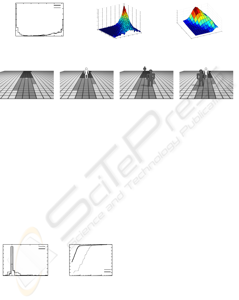
The result depicted by Fig. 9. shows that the
principled approach yields much better estimates of
the number of people than the baseline approach,
which triggers many false positives. When setting
the post-processing threshold so that both approaches
have about 10% of false negatives, our approach out-
performs the baseline one, by producing only about
0.06% of false positives instead of 0.81%. This re-
sult is depicted by the ROC curves of Fig. 9.b. Since
our method relies on a strong model and produces
very peaked occupancy probabilities, detection fail-
ures cases produce incorrect occupancy maps. This
explains the crossing of the ROC curves at very high
detection rates.
0
0.1
0.2
0.3
0.4
0.5
0.6
0.7
0.8
-5 0 5 10 15 20
Error in number of people detections
Baseline approach
Our approach
0
0.1
0.2
0.3
0.4
0.5
0.6
0.7
0.8
0.9
1
1e-04 0.001 0.01 0.1 1
True positives
False positives
Baseline approach
Our approach
(a) (b)
Figure 9: Comparing the performance of the baseline and
principled approaches. (a) Error distribution in the esti-
mate of the number of people present in the scene. (b) ROC
curves for the two methods. These graphs demonstrate that
the principled approach truly provides a better estimate of
the number of people present in the scene, and a better false
positives vs. false negatives ratio.
Indoor and Outdoor Sequences. Fig. 10 depicts
our results in the outdoor and indoor sequences. In
both cases, people are correctly detected in spite of
very real difficulties: In the outdoor images, there
are strong shadows, which could create problem for
methods based on background subtraction but do not
affect our results. The occlusions in the indoor im-
ages are very significant but are nevertheless handled
correctly, especially when one recalls that we do not
enforce any form of temporal consistency and treat
every time frame independently.
Thanks to the tree response model of Sec-
tion 3.3.2, we can retrieve occupancy maps from
the noisy classifier answers, even when using single
views as shown in last raw of Fig. 10. The procedure
used is the same as in the multi-view case, except that
we do no longer multiply tree’s answers from multi-
ple cameras in Equation 8. Occlusions are no longer
handled, as evidenced by the fact that a half-hidden
person in the second image is missed. Nevertheless,
the results remain meaningful.
5 CONCLUSIONS
We have shown that explicitly computing marginal
probabilities of target presence given classifier re-
sponses is more reliable and accurate than simply
averaging the responses across views for multi-view
PRINCIPLED DETECTION-BY-CLASSIFICATION FROM MULTIPLE VIEWS
381

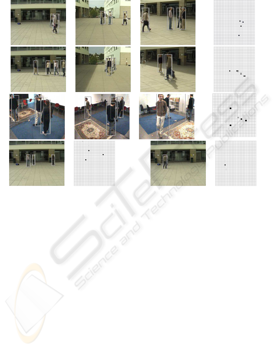
Figure 10: Results of our algorithm on real video sequences. Each one of the first three rows shows several views taken at
the same time instant from different angles. Boxes are located on local maxima of the estimated probabilities of occupancy.
The last column depicts the corresponding detection score map before thresholding. The last row shows two detection results
obtained from single images.
people detection purposes. This is especially true
in challenging situations with complex interactions
between true alarms due to occlusion and very low
metric accuracy in the classifier responses. Exper-
iments show that this method allows for a reduc-
tion of one order of magnitude of false positives.
As a result, we have been able to demonstrate reli-
able people detection at single time frames and with-
out having to impose any temporal consistency con-
straints. Finally, our approach to post-processing
multiple classifier outputs is generic and could be
applied to other detection-by-classification problems,
for which a model of the classifier response given
the true detection state is available, either directly or
through learning.
REFERENCES
Breiman, L. (1996). Bagging predictors. Machine Learn-
ing, 24(2):123–140.
Breiman, L., Friedman, J. H., Olshen, R. A., and Stone, C. J.
(1984). Classification and Regression Trees. Chap-
man & Hall, New York.
Dalal, N. and Triggs, B. (2005). Histograms of Oriented
Gradients for Human Detection. In CVPR.
Elfes, A. (1989). Occupancy Grids: A Probabilistic Frame-
work for Robot Perception and Navigation. PhD the-
sis, Carnegie Mellon University.
Fleuret, F. and Geman, D. (2002). Fast Face Detection with
Precise Pose Estimation. In CVPR.
Khan, S. and Shah, M. (2006). A multiview approach to
tracking people in crowded scenes using a planar ho-
mography constraint. In ECCV.
Leibe, B., Seemann, E., and Schiele, B. (2005). Pedestrian
detection in crowded scenes. In CVPR.
Mittal, A. and Davis, L. (2003). M2tracker: A multi-view
approach to segmenting and tracking people in a clut-
tered scene. IJCV.
Okuma, K., Taleghani, A., de Freitas, N., Little, J., and
Lowe, D. (2004). A boosted particle filter: multitarget
detection and tracking. In ECCV.
Viola, P. and Jones, M. (2001). Rapid Object Detection us-
ing a Boosted Cascade of Simple Features. In CVPR.
Viola, P., Jones, M., and D.Snow (2003). Detecting pedes-
trians using patterns of motion and appearance. In
ICCV.
Zhao, T. and Nevatia, R. (2001). Car detection in low reso-
lution aerial image. In ICCV.
VISAPP 2008 - International Conference on Computer Vision Theory and Applications
382