KLT TRACKING USING INTRINSIC AND EXTRINSIC CAMERA

PARAMETERS IN CONSIDERATION OF UNCERTAINTY

Michael Trummer, Joachim Denzler

Chair for Computer Vision, Friedrich-Schiller University of Jena, Ernst-Abbe-Platz 2, 07743 Jena, Germany

Christoph Munkelt

Optical Systems, Fraunhofer IOF, Albert-Einstein-Strasse 7, 07745 Jena, Germany

Keywords:

Feature tracking, epipolar geometry, 3D reconstruction.

Abstract:

Feature tracking is an important task in computer vision, especially for 3D reconstruction applications. Such

procedures can be run in environments with a controlled sensor, e.g. a robot arm with camera. This yields

the camera parameters as special knowledge that should be used during all steps of the application to improve

the results. As a ﬁrst step, KLT (Kanade-Lucas-Tomasi) tracking (and its variants) is an approach widely

accepted and used to track image point features. So, it is straightforward to adapt KLT tracking in a way

that camera parameters are used to improve the feature tracking results. The contribution of this work is an

explicit formulation of the KLT tracking procedure incorporating known camera parameters. Since practical

applications do not run without noise, the uncertainty of the camera parameters is regarded and modeled within

the procedure. Comparing practical experiments have been performed and the results are presented.

1 INTRODUCTION

1.1 Problem Statement and Motivation

The 3D reconstruction of objects from digital images

is a still unsolved problem, that has an important role

for many industrial applications. Especially hardware

systems containing a sensor mounted on a controlled

element (robot arm or equivalent), yielding positional

sensor parameters, are widely used (cf. (Kuehmstedt

et al., 2001)). Using this kind of set-up, it is shown

(Wenhardt et al., 2006) that the reconstruction result

can be improved, if the reconstruction process is em-

bedded in a next best view planning approach. But

without active illumination, all these reconstruction

methods suffer from the correspondence problem, i.e.

the identiﬁcation of image points mapped from one

3D world point.

For a pair of stereo images and known camera

(intrinsic and extrinsic) parameters, stereo matching

may be performed by scanning the other image’s cor-

responding horizontal line for one point within the

rectiﬁed image pair. But the above mentioned appli-

cations for 3D reconstruction provide video streams

by nature. Thus, feature point tracking is the way

most commonly used to collect image point corre-

spondences (like in (Wenhardt et al., 2006)) within the

image sequence. These feature point tracking meth-

ods, like KLT tracking, have been developed with re-

spect to the structure-from-motion approach. There-

fore, they ignore camera parameters.

All feature point tracking methods aim to ﬁnd

the mappings of one 3D world point into several im-

ages. Without any knowledge of the camera poses

or without using that knowledge, tracking algorithms

are bound to work appearance-based only. KLT track-

ing is doing so by minimizing the sum of squared er-

rors between the pixel intensity values of two patches

(small image regions). There is no reference to the

corresponding 3D world point at all, and hence, the

well-known motion drift problem (Rav-Acha and Pe-

leg, 2006) can occur. In addition, a lot of care has

to be taken for the selection of good features to track

(Shi and Tomasi, 1994).

Addressing the mentioned problems is the contri-

bution of this paper. This is done by explicitly incor-

porating knowledge about the camera (intrinsic and

extrinsic parameters) into the parameterization and

optimization process of KLT tracking. The search

space for patches in consecutive frames is restricted

346

Trummer M., Denzler J. and Munkelt C. (2008).

KLT TRACKING USING INTRINSIC AND EXTRINSIC CAMERA PARAMETERS IN CONSIDERATION OF UNCERTAINTY.

In Proceedings of the Third International Conference on Computer Vision Theory and Applications, pages 346-351

DOI: 10.5220/0001082403460351

 SciTePress

by the epipolar constraint. Hence, the above men-

tioned ways to establish point correspondences are

merged in order to create a new solution to the corre-

spondence problem for 3D reconstruction with a con-

trolled sensor.

The remainder of the paper is organized as fol-

lows. In section 2 the parameterization and optimiza-

tion process of KLT tracking is described. The incor-

poration of the epipolar constraint (by using intrinsic

and extrinsic camera parameters as prior knowledge)

is demonstrated in section 3. Section 4 shows, how

the uncertainty of the epipolar geometry is given at-

tention to and modeled within the extended tracker.

Experimental results are demonstrated in section 5,

and the paper is concluded in the last section.

1.2 Literature Review

The original idea of tracking features by an itera-

tive optimization process was presented by Lucas

and Kanade in (Lucas and Kanade, 1981). Since

then a rich variety of adaptations and extension has

been published, giving rise to surveys like (Baker and

Matthews, 2004). (Fusiello et al., 1999) deal with the

removal of spurious corespondences by using robust

statistics. The problem of reselection of the template

image is dealt with in (Zinsser et al., 2005).

Since these modiﬁcations and extensions are inde-

pendent from applying camera parameters, only very

few of them are mentioned. For more information

the reader may be referred to (Baker and Matthews,

2004).

2 KLT TRACKING

In this section the basic equations of KLT tracking are

derived and summarized as far as needed for the re-

mainder of the paper. This can also be found in (Baker

and Matthews, 2004).

Under the assumptions of constant image bright-

ness (see (Cox et al., 1995)) and a small baseline

between consecutive frames, the pixel-wise sum of

squared intensity differences between small image re-

gions (patches) T(x) from the ﬁrst image and I(x)

from the second image deﬁnes an error ε. The func-

tions T(x) and I(x) yield the intensity values at pixel

position x = (x, y)

in the respective image region P.

Now, the error ε is parameterized by a vector p. The

entries of this vector are used for the deﬁned geomet-

rical warping W(x, p) from T(x) to I(W(x, p)). Thus,

the error is

ε(p) =

∑

x∈P

(I(W(x, p))− T(x))

. (1)

The warping function W(x, p) may perform differ-

ent geometrical transformations. Common choices

are pure translation (thus, p = (p

, p

)

containing

two parameters for translation within the image plane,

namely in image x- and y-direction), afﬁne transfor-

mation (six parameters) or projective transformation

(eight parameters).

Within the iterative optimization process, where

an initial allocation of p is already known, equation

(1) is reparameterized with ∆p to

ε(∆p) =

∑

x∈P

(I(W(x, p+ ∆p))− T(x))

, (2)

also known as compositional approach. In order to

solve for ∆p, two ﬁrst-order Taylor approximations

are performed, yielding (for details the reader is re-

ferred to (Baker and Matthews, 2004))

′

(∆p) =

∑

x∈P

(I(W(x, p)) + ∇I

∂W(x, p)

∂p

∆p− T(x))

(3)

where

∂W(x,p)

∂p

is the Jacobian of W(x, p), with

ε(∆p) ≈ ε

′

(∆p). For the purpose of minimization, the

ﬁrst derivative of equation (3) is set to zero. Hence,

the optimization rule is

∆p = H

−1

∑

x∈P



∇I

∂W(x, p)

∂p



(T(x) − I(W(x, p)))

(4)

with the Hessian

H =

∑

x∈P



∇I

∂W(x, p)

∂p





∇I

∂W(x, p)

∂p



. (5)

By equation (4) an optimization rule is deﬁned for

computing p

i+1

from p

, namely p

i+1

= p

+ ∆p.

3 USING INTRINSIC AND

EXTRINSIC CAMERA

PARAMETERS

In this section the reparameterization of the warp-

ing function W(x, p) by using camera parameters

(intrinsic and extrinsic) as prior knowledge is de-

scribed. The additional knowledge is used to com-

pute the epipolar geometry (cf. (Hartley and Zisser-

man, 2003)) of consecutive frames. Then the transla-

tional part of the warping function is modiﬁed so that

the template patch can only be moved along the cor-

responding epipolar line. With respect to clarity and

KLT TRACKING USING INTRINSIC AND EXTRINSIC CAMERA PARAMETERS IN CONSIDERATION OF

UNCERTAINTY

347

w.l.o.g. the warping function is assumed to perform a

pure translation, since the modiﬁcations do not affect

the afﬁne or projectivepart of the transformation. The

treatment of afﬁne and projective parameters remains

the same as for the standard KLT tracker.

For the computation of the fundamental matrix

F from camera parameters the reader is referred to

(Hartley and Zisserman, 2003). Once calculated, the

position of a point x in the ﬁrst image can be restricted

to the corresponding epipolar line l = (l

, l

)

the second image. The epipolar line l is given by

l = F

x with

x = (x, y, 1)

. A parameterized form of

this line is

l(λ) =



−l



+ λ



−l



(6)

with parameter λ. Thus, for pure translation the new

epipolar warping function is given by

(x, p) =



−l

− λl

λl



, (7)

using l = F

x and p = λ. In the case of l

being

close to zero, another parameterization of l has to be

used. Equation (7) shows the reparameterization of

the translational transformation regarding the epipolar

constraint. The Jacobian of this expression is simply

∂W

(x, p)

∂p

∂W

E,x

(x,p)

∂λ

∂W

E,y

(x,p)

∂λ



−l



. (8)

Using equation (8) in the optimization rule from

equations (4) and (5), the adaptation to the case of

known camera parameters is reached. For the mo-

ment, the translation of a pixel between two frames

is strictly limited to the movement along the corre-

sponding epipolar line (expressed by parameter λ), re-

ducing the optimization search space by one degree of

freedom.

4 IN CONSIDERATION OF

UNCERTAINTY

Up to now, the warping function for one pixel is only

allowing for movements on the corresponding epipo-

lar line. But with respect to noisy camera parameters

and to discretization, a possible deviation from the

epipolar line has to be modeled. This section shows a

way to incorporate uncertainty into the parameteriza-

tion and into the optimization process from equation

(4).

For the mentioned, obvious reasons the restriction

of moving only along the epipolar line has to be soft-

ened. This can be achieved by allowing movement

perpendicular to the epipolar line. But, with these

two linearly independent directions, the search space

again covers the whole image plane, which seems to

neutralize any advantages reached by the reduction of

the number of parameters. Consequently, some mech-

anism to control the single translational parts (perpen-

dicular to / along the epipolar line) has to be added.

This is achieved by a weighting factor w ∈ [0, 1],

called epipolar weight, controlling the amounts of ac-

cepted parameter changes.

With respect to uncertainty the modiﬁed epipolar

warping function is

(x, p) =



−l

− λ

+ λ



, (9)

with l = F

x, p = (λ

, λ

)

and the Jacobian

∂W

(x, p)

∂p

∂W

EU,x

(x,p)

∂λ

∂W

EU,x

(x,p)

∂λ

∂W

EU,y

(x,p)

∂λ

∂W

EU,y

(x,p)

∂λ



−l



. (10)

Applying this to the rule from equations (4) and (5),

nearly the original optimization is performed, but

with the exception of translating along and perpen-

dicular to the corresponding epipolar line and not in

image x- and y-direction (for the general case). The

epipolar constraint respecting uncertainty is achieved

by adding to the optimization rule a weighting matrix



w 0

0 1− w



(11)

that controls the amount (within each dimension) of

the calculated ∆p that is accepted, ﬁnally. The modi-

ﬁed optimization rule is

∆p

EU,w

= A

−1

(12)

with H

given by expression (5) with the substitu-

tion from equation (10) and

∑

x∈P



∇I

∂W

(x, p)

∂p



(T(x)−I(W

(x, p))).

(13)

By this speciﬁcation, the change of translational

parameters is optimized with respect to the epipo-

lar geometry. Changes along the epipolar line are

accepted with weight w (perpendicular with weight

VISAPP 2008 - International Conference on Computer Vision Theory and Applications

348

1 − w) within each optimization step. For the hypo-

thetical case of a perfectly accurate epipolar geome-

try, w = 1 could be used, resulting in the optimization

rule described in section 3. The automatic computa-

tion of w has not been explored, yet. There might be

a way to yield w with respect to the uncertainty of the

epipolar line calculated from noisy camera parame-

ters.

5 EXPERIMENTAL RESULTS

This section shows experimental results. The stan-

dard KLT tracker is compared to the modiﬁed tracker

described in this work in terms of tracking accuracy

and mean trail length of tracked points in an image

sequence. As warping function both trackers use the

respective variants of pure translation (x-/y-direction,

-/λ

-direction). The performance of the modiﬁed

tracker is tested with respect to the epipolar weight w.

5.1 Trail Length Evaluation

For this experiment an image sequence has been

recorded. The calibrated camera was mounted on the

hand of a Staeubli RX90L robot arm providing the

extrinsic parameters. The image sequence consisted

of 21 frames, one for the initialization of the tracker

and 20 for tracking. The ﬁgures 1 to 3 show some

of the 100 features selected (pictures are cut and en-

larged for visibility reasons) and two tracking steps.

The images are taken from the test run with w = 0.9

set.

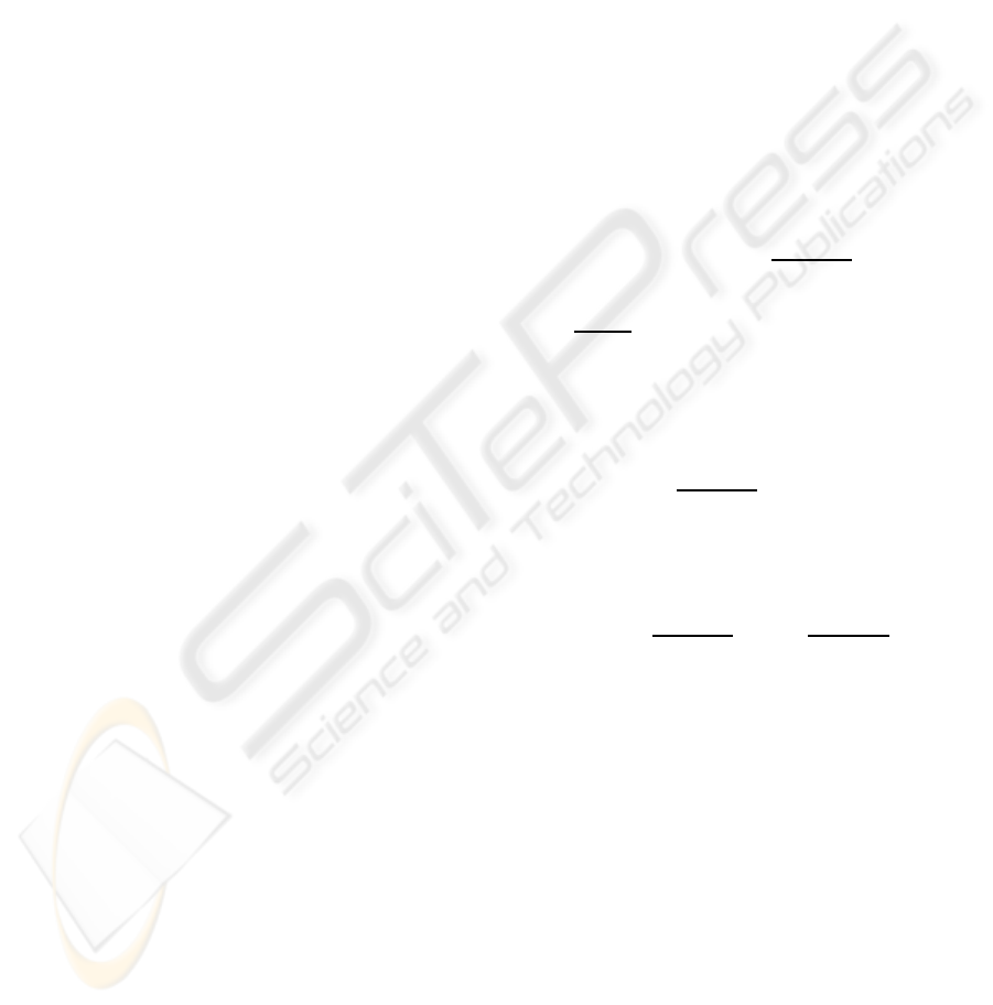
Figure 1: Initial frame with 100 image features selected.

The ﬁgures show partially different positions of

the tracked features. This effect is quantiﬁed in the

next subsection.

For each feature point the trail length (number

of frames in which the point could be tracked) was

Figure 2: Frame 9. Tracked points by standard KLT marked

by light green crosses. Yellow diamonds indicate points of

the modiﬁed tracker (w = 0.9).

Figure 3: Frame 20.

stored. From these values the mean trail length and

the variance for all points were computed. The results

are shown in tables 1 and 2.

Table 1: Mean trail lengths and variances with respect to w.

Values for standard tracker: mean 16.07 frames (fr), vari-

ance 27.83 frames

epipolar weight w 0.5 0.6 0.7

mean trail length (fr) 15.96 16.16 16.18

variance (fr

) 28.12 26.97 27.11

Table 2: Continuing table 1.

epipolar weight w 0.8 0.9 0.95

mean trail length (fr) 16.10 16.00 16.04

variance (fr

) 26.99 27.74 27.64

The values from tables 1 and 2 show comparable

performance for the aspect of mean trail length. For

w = 0.7 the mean trail length produced by the mod-

iﬁed tracker is about one percent longer then by the

standard KLT tracker.

KLT TRACKING USING INTRINSIC AND EXTRINSIC CAMERA PARAMETERS IN CONSIDERATION OF

UNCERTAINTY

349

5.2 Accuracy Evaluation

Especially with respect to 3D reconstruction, another

important characteristic of a feature tracker is the ac-

curacy of the tracked feature points. To compare the

accuracy of the modiﬁed tracker to the standard KLT

tracker, ground truth information has been generated

for an image pair (ﬁgures 4 and 5). The ground truth

correspondences in the second image were blindly

(without knowledge about the tracking results) hand-

marked. Extrinsic camera parameters were calculated

by the method proposed in (Trummer et al., 2006).

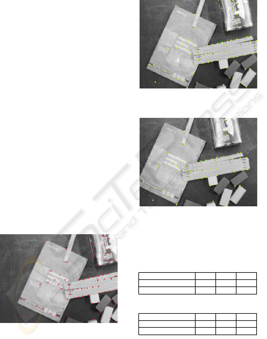
Figure 4: First frame with 100 features selected.

Figure 5: Second frame. Again, tracked points by standard

KLT marked by light green crosses. Yellow diamonds indi-

cate points of the modiﬁed tracker (w = 0.5).

Especially along edges the results of the track-

ers differ from each other. The tracking accuracy is

expressed in terms of the mean error distance of a

tracked point from its ground truth correspondence.

The variance is also given. Tables 3 and 4 show the

results for different values of w.

With the modiﬁed tracker, for each allocation of w

the mean error distance is up to one pixel smaller than

Table 3: Mean error distance with respect to w. Values

for standard tracker: mean 5.84 pixels (px), variance 51.40

pixels

epipolar weight w 0.5 0.6 0.7

mean error distance (px) 4.78 4.69 4.97

variance (px

) 30.52 32.19 39.80

Table 4: Continuing table 3.

epipolar weight w 0.8 0.9 0.95

mean error distance (px) 4.89 5.37 5.39

variance (px

) 48.14 52.32 55.98

for the standard KLT tracker. An interesting point is

the error value for w = 0.5. In that case, the modiﬁed

optimization in principal does the same as the stan-

dard one. Only the optimization step size is half as

wide (w = 0.5) and the translation is optimized along

directions λ

and λ

(along/perpendicular to the re-

spective epipolar line). But, already this reparame-

terization of the translation directions has positive in-

ﬂuence on the tracking accuracy. The large variances

are due to point features along edges, where larger er-

rors may occur. But also this negative effect of the

the well-known aperture problem is constricted, if w

is chosen properly. With feature points being tracked

more accurately, the input data for 3D reconstruction

and, thus, the reconstruction result will beneﬁt.

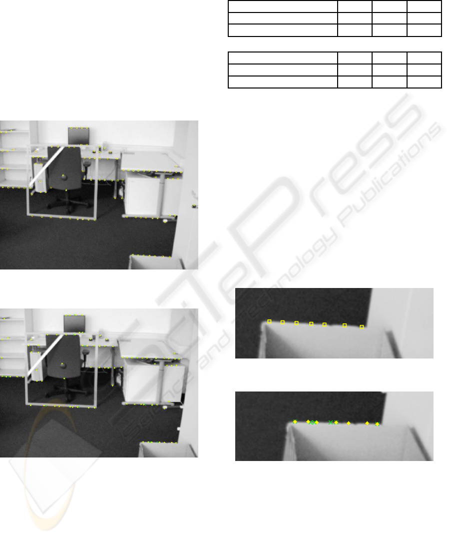
Figure 6: Close-up from ﬁgure 4 showing initial features

along edge.

Figure 7: Tracking results as close-up from ﬁgure 5. Stan-

dard tracker (points marked by light green crosses) lost one

point, some of the others are drifted along the edge. Mod-

iﬁed tracker (yellow diamonds) found all points and pre-

served point alignment.

The ﬁgures 6 and 7 demonstrate more clearly the

differences between the results of the compared track-

ers. By incorporating the epipolar constraint with re-

gard to uncertainty, the modiﬁed tracker was able to

ﬁnd one more point in the illustrated region and to

keep a better alignment of the tracked feature points.

VISAPP 2008 - International Conference on Computer Vision Theory and Applications

350

The mean error distance was up to 20 percent smaller

(for w = 0.6) using the modiﬁed tracker.

6 CONCLUSIONS AND

OUTLOOK

In this paper we showed a method to modify the well-

known KLT tracker incorporating knowledge about

the extrinsic and intrinsic camera parameters. The ad-

ditional prior knowledge is utilized to reparameterize

the warping function. With respect to noise in prac-

tical applications, uncertainty is modeled within the

optimization rule. While the mean trail length could

only be improved very slightly, the experiments per-

formed show a better accuracy when using the mod-

iﬁed tracker. Remarkable is the fact that the epipolar

optimization directions alone have a positive effect on

the tracking result.

For the future, this modiﬁcation of the KLT

tracker offers lots of further topics to be investigated.

Setting the weighting factor w to a certain value may

be replaced by an automatic detection concerning the

amount of uncertainty of the camera parameters. We

also think about changing w during the optimization

process.

Another step is the concurrent improvement of ac-

curacy and trail length. At the current stage, accu-

racy is addressed already. When aiming at longer trail

lengths, a closer look at the reasons of losing a feature

has to be taken. One of these reasons, surely, is a too

large error measured (cf. expression (1)) between cor-

responding patches. That means, the selected trans-

formation is not able to model all changes between

the patches within the error bound set. But with re-

gard to the (soft) epipolar constraint of the modiﬁed

tracker, this error bound may be raised without the op-

timization process losing its way. Another possibility

to be explored is random jumping along the epipolar

line, when a feature is lost.

REFERENCES

Baker, S. and Matthews, I. (2004). Lucas-kanade 20 years

on: A unifying framework. International Journal of

Computer Vision, 56:221–255.

Cox, I., Roy, S., and Hingorani, S. L. (1995). Dynamic

histogram warping of image pairs for constant image

brightness. IEEE International Conference on Image

Processing, 2:366–369.

Fusiello, A., Trucco, E., Tommasini, T., and Roberto, V.

(1999). Improving feature tracking with robust statis-

tics. Pattern Analysis and Applications, 2:312–320.

Hartley, R. and Zisserman, A. (2003). Multiple View Geom-

etry in computer vision, Second Edition. Cambridge

University Press.

Kuehmstedt, P., Notni, G., Hintersehr, J., and Gerber, J.

(2001). Cad-cam-system for dental purpose – an in-

dustrial application. In The 4th International Work-

shop on Automatic Processing of Fringe Patterns.

Lucas, B. and Kanade, T. (1981). An iterative image regis-

tration technique with an application to stereo vision.

In Proceedings of 7th International Joint Conference

on Artiﬁcial Intelligence.

Rav-Acha, A. and Peleg, S. (2006). Lucas-kanade without

iterative warping. In Proceedings of 2006 IEEE Inter-

national Conference on Image Processing.

Shi, J. and Tomasi, C. (1994). Good features to track. In

Proceedings of IEEE Computer Society Conference

on Computer Vision and Pattern Recognition.

Trummer, M., Denzler, J., and Suesse, H. (2006). Precise 3d

measurement with standard means and minimal user

interaction – extended single-view reconstruction. In

Proceedings of 17th International Conference on the

Application of Computer Science and Mathematics in

Architecture and Civil Engineering.

Wenhardt, S., Deutsch, B., Hornegger, J., Niemann, H., and

Denzler, J. (2006). An information theoretic approach

for next best view planning in 3-d reconstruction. In

The 18th International Conference on Pattern Recog-

nition.

Zinsser, T., Graessl, C., and Niemann, H. (2005). High-

speed feature point tracking. In Proceedings of Con-

ference on vision, Modeling and Visualization.

KLT TRACKING USING INTRINSIC AND EXTRINSIC CAMERA PARAMETERS IN CONSIDERATION OF

UNCERTAINTY

351