
A MAXIMUM LIKELIHOOD SURFACE NORMAL ESTIMATION
ALGORITHM FOR HELMHOLTZ STEREOPSIS
Jean-Yves Guillemaut
1
, Ondˇrej Drbohlav
2
, John Illingworth
1
and Radim
ˇ
S´ara
3
1
Centre for Vision, Speech and Signal Processing, University of Surrey, Guildford, Surrey, GU2 7XH, UK
2
Visual Cognitive Systems Laboratory, University of Ljubljana, Trˇzaˇska 25, SI-1001 Ljubljana, Slovenia
3
Center for Machine Perception, Czech Technical University, Karlovo n´amˇest´ı 13, Prague 2, Czech Republic
Keywords:
Helmholtz Stereopsis, Photometry, Image-Based Object Reconstruction.
Abstract:
Helmholtz stereopsis is a relatively recent reconstruction technique which is able to reconstruct scenes with
arbitrary and unknown surface reflectance properties. Conventional implementations of the method estimate
surface normal direction at each surface point via an eigenanalysis, thereby optimising an algebraic distance.
We develop a more physically meaningful radiometric distance whose minimisation is shown to yield a Maxi-
mum Likelihood surface normal estimate. The proposed method produces more accurate results than algebraic
methods on synthetic imagery and yields excellent reconstruction results on real data. Our analysis explains
why, for some imaging configurations, a sub-optimal algebraic distance can yield good results.
1 INTRODUCTION
Most image-based reconstruction techniques assume
that the surface reflectance of the scene is known or
follows a parametric model. Conventional binocu-
lar stereo relies on the assumption that the scene is
Lambertian, i.e. the appearance of a surface point
is independent of the viewing direction. Photomet-
ric stereo can cope with non Lambertian reflectance
models, but still relies on a known parametric surface
reflectance model. Shape-from-silhouette does not
make any assumption on surface reflectance but the
obtainable reconstruction is only approximate (lim-
ited to the visual hull) and often requires capture of a
large number of images. In contrast, Helmholtz stere-
opsis (HS), introduced in (Magda et al., 2001; Zickler
et al., 2002a), has the unique property of being able to
reconstruct objects with arbitrary and unknown sur-
face reflectance properties.
HS is based on the Helmholtz reciprocity princi-
ple, which states that at any surface point the sur-
face reflectance, represented by its bidirectional re-
flectance distribution function (BRDF) (Nicodemus
et al., 1977), remains unchanged when the incident
and reflected directions are interchanged. The method
requires a camera and a point light source whose po-
sitions can be interchanged in order to produce recip-
rocal pairs of images. The method was first imple-
mented in the case of a general multi-camera setup
(Magda et al., 2001; Zickler et al., 2002a; Zickler
et al., 2002b) and then in a binocular configuration
(Tu and Mendonc¸a, 2003; Zickler et al., 2003b). In
(Zickler et al., 2003a; Zickler, 2006), HS was later ex-
tended to uncalibrated cameras. Other research con-
centrated on improving the accuracy of HS by radio-
metric calibration (Jank´o et al., 2004), as well as gen-
eralising the method to structured and strongly tex-
tured surfaces (Guillemaut et al., 2004). Applications
of the Helmholtz reciprocity principle have also been
considered in the contexts of surface registration (Tu
et al., 2003) and computer graphics (Sen et al., 2005).
HS produces a scene reconstruction consisting of
a depth estimate and surface normal estimate at each
pixel in a reference view. This yields a 2.5D repre-
sentation of the scene from which the surface can be
extracted by integration of the normal field. Accu-
rate surface normal estimation at each pixel is there-
fore critical. In previous implementations, reciprocal
pairs of images were used to define a set of linear con-
straints, from which the normal is estimated by find-
ing the vector best satisfying all constraints. Singular
value decomposition (SVD) (Press et al., 1992) has
been used for such task, because it allows computa-
tion of a global solution at a low computational cost.
352
Guillemaut J., Drbohlav O., Illingworth J. and Šára R. (2008).
A MAXIMUM LIKELIHOOD SURFACE NORMAL ESTIMATION ALGORITHM FOR HELMHOLTZ STEREOPSIS.
In Proceedings of the Third International Conference on Computer Vision Theory and Applications, pages 352-359
DOI: 10.5220/0001083203520359
Copyright
c
SciTePress

A drawback however is that the algebraic error func-
tion thus defined often lacks a physical meaning and
is not optimum in a statistical sense.
In contrast, in this paper we propose to formu-
late the surface normal estimation problem in terms
of minimising a distance that we call the radiomet-
ric distance. This distance is physics-based and mea-
sures the intensity modification to be applied in order
to satisfy exactly the Helmholtz reciprocity constraint
at a surface point. Under standard Gaussian image
noise conditions, its minimisation yields a maximum
likelihood (ML) surface normal estimate. We demon-
strate that the computation of this optimum solution
can be done efficiently by minimising a non-linear
cost function with two variables only. The proposed
algorithm also incorporates treatment of image satu-
ration, a phenomenon which has often been ignored
in previous work.
The paper is structured as follows. We start by
giving an overview of HS, where we describe the
conventional surface normal estimation algorithm. In
the following section, we propose a novel radiomet-
ric distance and an efficient minimisation algorithm
for deriving the surface normal. Finally, we present
results on synthetic and real imagery, and conclude.
2 OVERVIEW OF HELMHOLTZ
STEREOPSIS
v
r
v
l
O
r
O
l
n
X
v
r
v
l
O
r
O
l
n
X
Figure 1: A reciprocal configuration.
Let us consider the configuration illustrated in Fig-
ure 1. O
l
and O
r
are two points in space and X is a
surface point. We denote by d
l
= kO
l
− Xk and d
r
=
kO
r
− Xk the distances from O
l
and O
r
respectively
to X, and define v
l
=
1
d
l
(O
l
−X) and v
r
=
1
d
r
(O
r
−X),
which represent the unit vectors pointing from X to O
l
and O
r
respectively. The surface normal at X is rep-
resented by the unit vector n. The BRDF f(X, u, v) at
X is by definition the ratio of the outgoing radiance
along the direction v to the incident irradiance along
the direction u. If we position an isotropic light source
of intensity κ at O
l
and a camera at O
r
, the pixel in-
tensity
1
i
r
observed by the camera is:
i
r
= f(X, v
l
, v
r
)
v
l
· n
d
2
l
κ. (1)
If the positions of the light source and the camera are
now swapped, an analogous formula is obtained for
the radiance i
l
observed by the camera at position O
l
:
i
l
= f(X, v
r
, v
l
)
v
r
· n
d
2
r
κ. (2)
The two images captured by such cameras form a
reciprocal pair. The Helmholtz reciprocity princi-
ple states that f(X, v
l
, v
r
) = f(X, v
r
, v
l
). Combin-
ing Eq. (1) and Eq. (2), and denoting s
l
=
1
d
2
l
v
l
and
s
r
=
1
d
2
r
v
r
, we obtain (Zickler et al., 2002b):
(i
l
s
l
− i
r
s
r
) · n = 0. (3)
The vector (i
l
s
l
− i
r
s
r
) must lie in the tangent plane
at the surface point and the normal vector n can, in
principle, be estimated from two or more such vectors
(derived from two or more reciprocal pairs).
2.1 Surface Points Identification
Surface points are represented by a depth value at
each pixel in a reference view. If at least N ≥ 3 con-
straints defined by Eq. (3) are available (one per recip-
rocal pair of images), it is possible to define a measure
for identifying such points. At each candidate surface
point, we can form the following system of N ≥ 3
equations (Zickler et al., 2002b):
W n = 0 with (4)
W =
i
l
1
s
l
1
− i
r
1
s
r
1
, . . . , i
l
n
s
l
n
− i
r
n
s
r
n
⊤
.
The distribution of row vectors in W is then used to
identify surface points as follows. If the intensities
used for constructing the matrix W come from a sur-
face point, these vectors must be coplanar and, there-
fore, the matrix W must be of rank 2. If the point
is not a surface point, the rows of the matrix W are
likely not to conform to this constraint. In practice,
the rank 2 constraint is never exactly satisfied, even at
surface points, because of image noise. For this rea-
son, an alternative measure of rank, which we call the
support measure, is defined by:
s = 1−
σ
3
σ
2
, (5)
1
We adopt the convention that the pixel intensity is equal
to the scene radiance. This is usually a reasonable assump-
tion for high quality cameras. If it is not the case, radio-
metric calibration can be performed in order to meet this
requirement (Jank´o et al., 2004).
A MAXIMUM LIKELIHOOD SURFACE NORMAL ESTIMATION ALGORITHM FOR HELMHOLTZ STEREOPSIS
353

where σ
2
and σ
3
denote the second and third singular
values of W . It is assumed here that the SVD of W is
written in the form:
W = UDV
⊤
with (6)
D = diag(σ
1
, σ
2
, σ
3
) and σ
1
≥ σ
2
≥ σ
3
≥ 0.
The measure defined in Eq. (5) is strictly equivalent to
the measure defined in (Zickler et al., 2002b), but has
the advantage of normalising the value of the support
measure between 0 and 1, a value close to 1 corre-
sponding to a high chance of the point being located
on a surface.
The conditions given in Eq. (4) are necessary, but
not sufficient, for a point to be located at the surface.
It can, therefore, happen that the support measure de-
fined in Eq. (5) is large although the point does not be-
long to the surface. A possibility to resolve this ambi-
guity is to optimise the measure over a small window
instead of a single pixel, assuming that the surface
can be locally represented by a fronto-parallel pla-
nar patch as in (Zickler et al., 2002b). Surface points
are then identified by maximising the support mea-
sure along each ray in the reference image sampled
with regular depth increments. This yields a 2.5D sur-
face reconstruction represented by a depth map. Typi-
cally the depth map obtained may be noisy, but a more
accurate estimate of the object geometry can be ob-
tained by computing the surface normal at each point
and then integrating the obtained normal field - this is
a standard procedure used in photometric stereo.
2.2 Surface Normal Estimation
Given some identified surface points, previous ap-
proaches (Magda et al., 2001; Zickler et al., 2002b)
have estimated the normal n at each point as the third
singular vector, i.e. the last column vector of V , from
the SVD of W expressed in Eq. (6). It can be shown
(see e.g. (Hartley, 1997)) that the solution obtained is
the vector n which minimises
kW · nk
2
=
∑
j
[(i
l
j
s
l
j
−i
r
j
s
r
j
)·n]
2
subject to knk = 1. (7)
This cost function can be written in the form
∑
j
d
alg
(n, i
l
j
, i
r
j
, s
l
j
, s
r
j
)
2
, (8)
where d
alg
denotes the algebraic distance
d
alg
(n, i
l
j
, i
r
j
, s
l
j
, s
r
j
)
2
= [(i
l
j
s
l
j
− i
r
j
s
r
j
) · n]
2
(9)
= ki
l
j
s
l
j
− i
r
j
s
r
j
k
2
cos
2
α
j
.
In this expression, α
j
denotes the angle between the
vector (i
l
j
s
l
j
− i
r
j
s
r
j
) and the surface normal n. The
term cos
2
α
j
is small when the constraint Eq. (3) is
close to be satisfied and, conversely, large when the
constraint is far from being satisfied; this term there-
fore intuitively corresponds to an entity to be min-
imised. However, the physical interpretation of the
scaling factor ki
l
j
s
l
j
− i
r
j
s
r
j
k
2
is not obvious. The in-
fluence of this term could be eliminated by normalis-
ing the rows of W to unit values, however it is pos-
sible that these coefficients play an important role by
attenuating the contribution of measurements corre-
sponding to low intensities or cameras/light sources
located far away from the scene point. In any case, the
SVD-based solutions, considered in previous works
mainly for simplicity reasons, did not explicitly ad-
dress the nature of errors affecting the measurements,
and therefore, have no guarantee of optimality. In the
next section, we propose a novel measure, which we
prove to be optimum under the assumption that errors
affecting the normal computation are due to Gaussian
noise in intensity measurements.
3 RADIOMETRIC CONSTRAINT
3.1 Definition
Since the fundamental entities observed are image in-
tensities (or equivalently, radiances), it is a natural
choice to perform the minimisation directly in the
space of radiances. We define an optimum solution
by searching for the surface normal n and the intensity
pairs {
ˆ
i
l
j
,
ˆ
i
r
j
}
j
which minimise the cost function
2
:
∑
j
(
ˆ
i
l
j
− i
l
j
)
2
+ (
ˆ
i
r
j
− i
r
j
)
2
(10)
subject to ∀ j (
ˆ
i
l
j
s
l
j
−
ˆ
i
r
j
s
r
j
) · n = 0.
This cost function measures the correction to be made
in the intensities observed in each reciprocal pair of
images in order to fulfil exactly the constraints defined
in Eq. (4). If we assume that the error in geometric
calibration of the camera and light source is negligi-
ble compared to the intensity measurement error, and
that the intensity measurement errors are independent
and follow Gaussian distributions, the resulting cost
function defines a sum of squared errors affected only
by Gaussian noise, and its minimisation leads to an
ML estimate.
After elimination of the constraints by substitution
2
Note that for conciseness, we use the notation {
ˆ
i
l
j
}
j
in-
stead of {
ˆ
i
l
j
}
j∈{1,...,N}
. Whenever the range has been omit-
ted in this paper, it should be understood that the range is
{1, . . . , N}.
VISAPP 2008 - International Conference on Computer Vision Theory and Applications
354

into the cost function, we obtain:
∑
j
[(
ˆ
i
l
j
− i
l
j
)
2
+ (
s
l
j
· n
s
r
j
· n
ˆ
i
l
j
− i
r
j
)
2
], (11)
where the variables to optimise are n and {
ˆ
i
l
j
}
j
. This
defines a priori a complex minimisation problem with
3 + N unknowns, N being the number of reciprocal
image pairs. We demonstrate in the appendix that this
minimisation problem can be simplified into an equiv-
alent problem where n is the only unknown. The ob-
tained cost function to minimise is
∑
j
d
rad
(n, i
l
j
, i
r
j
, s
l
j
, s
r
j
)
2
, (12)
where d
rad
denotes the novel radiometric distance in-
troduced and defined by:
d
rad
(n, i
l
j
, i
r
j
, s
l
j
, s
r
j
)
2
=
[(i
l
j
s
l
j
− i
r
j
s
r
j
) · n]
2
(s
l
j
· n)
2
+ (s
r
j
· n)
2
. (13)
This defines a simple minimisation problem with only
two degrees of freedom (the norm of n must be one).
The solution can be computed using a non-linear opti-
misation algorithm such as the Levenberg-Marquardt
algorithm (Press et al., 1992). The algorithm can be
initialised with the result of the SVD solution and usu-
ally converges rapidly after only a few iterations. To
be physically valid, the solution obtained must sat-
isfy the visibility constraints stating that s
l
· n > 0 and
s
r
· n > 0. Although these constraints can be enforced
during minimisation of the cost function, we found it
simpler and sufficient to verify that the visibility con-
straints are satisfied after convergence of the search
algorithm. Note that these constraints also guarantee
that the denominators of the equations considered in
this section and in the appendix are non-zero.
3.2 Comparison with the Algebraic
Constraint
From Eq. (9) and Eq. (13), we have:
d
rad
(n, i
l
j
, i
r
j
, s
l
j
, s
r
j
)
2
= (14)
1
(s
l
j
· n)
2
+ (s
r
j
· n)
2
d
alg
(n, i
l
j
, i
r
j
, s
l
j
, s
r
j
)
2
.
Although the interpretation of the multiplicative fac-
tor relating the two measures does not seem imme-
diately obvious, it is apparent that the difference be-
tween the two constraints is due only to the positions
of the camera and light source relatively to the sur-
face point, and does not involve the measured inten-
sities. The two measures will produce identical nor-
mal estimates wheneverthe term (s
l
j
·n)
2
+(s
r
j
·n)
2
is
constant for all j. One particular situation when this
occurs in practice is for horizontal surfaces located at
the centre of the turntable used in our experimental
set up (see Section 4.2).
3.3 Treatment of Image Saturation
Specularities can be difficult to capture due to the lim-
ited range of the camera sensor and often result in sat-
urated pixels. This affects the constraints previously
defined because the measured intensities are no longer
proportional to the true radiance. So far, very little at-
tention has been paid to this problem apart from (Tu
and Mendonc¸a, 2003) where a solution is reported in
the case of binocular HS. We propose a similar treat-
ment of image saturation in the multiocular case, and
adapt the radiometric distance accordingly.
As in (Tu and Mendonc¸a, 2003), we observe that
when a saturation is present in a reciprocal pair of
images (usually it is observed simultaneously in both
images at reciprocal positions), the normal bisects the
incident and emerging rays, and we have
(
1
ks
l
j
k
s
l
j
−
1
ks
r
j
k
s
r
j
) · n = 0. (15)
This constraint must replace Eq. (3) whenever a sat-
uration is observed. In this case, the appropriate row
of W in Eq. (4) is replaced by (
i
sat
ks
l
j
k
s
l
j
−
i
sat
ks
r
j
k
s
r
j
)
⊤
before computing the SVD, and for the radiometric
constraint, Eq. (13) is replaced by:
d
rad
(n, i
l
j
, i
r
j
, s
l
j
, s
r
j
)
2
= [(
i
sat
ks
l
j
k
s
l
j
−
i
sat
ks
r
j
k
s
r
j
) · n]
2
.
(16)
In these expressions, the value i
sat
, representing the
pixel saturation intensity value, is necessary to guar-
antee that the dimension is the same as in Eq. (3) or
Eq. (13). This distance is similar to the cost function
defined by Tu and Mendonc¸a in (Tu and Mendonc¸a,
2003) in the case of binocular HS.
4 RESULTS
4.1 Synthetic Data
We conduct a simple experiment to compare the per-
formances of the proposed radiometric distance with
the algebraic distance. Two implementations are con-
sidered for the algebraic distance described in Sec-
tion 2.2. The first one, which was adopted in (Zick-
ler et al., 2002b), uses the matrix W as defined in
Eq. (4) for computation of the SVD and is called
unnormalised algebraic; the second implementation
proceeds similarly but with rows normalised to unit
values and is called normalised algebraic. The issue
of normalisation has been discussed earlier in Sec-
tion 2.2. We consider the reconstruction of a sur-
face patch with ground truth normal n whose BRDF
A MAXIMUM LIKELIHOOD SURFACE NORMAL ESTIMATION ALGORITHM FOR HELMHOLTZ STEREOPSIS
355

is modelled by the modified Phong reflectance model
described in (Lewis, 1994; Lafortune and Willems,
1994). The model represents the BRDF as the sum of
a diffuse component and a specular component:
f
n,k
d
,k
s
(X, v
l
, v
r
) = k
d
1
π
+ k
s
n+ 2
2π
cos
n
α, (17)
where α denotes the angle between the perfect spec-
ular reflective direction and the emerging direction.
The three parameters n, k
d
and k
s
represent respec-
tively the specular exponent (large values result in
sharper specular reflections), the diffuse reflectivity
and the specular reflectivity. In our experiment, we
considered the values n = 40, k
d
= 0.4 and k
s
= 0.05.
There exist more sophisticated models which could
have been considered, such as the one described in
(Cook and Torrance, 1982), but it is important to note
that there is no “perfect” model, all existing models
being restricted to a particular class of surfaces. Also
it was observed in Section 3.2 that the relative perfor-
mance of algebraic and radiometric algorithms should
be independent of the surface model, therefore the
choice of the reflectance model is not critical as long
as it is physically plausible. We chose the modified
Phong model because it is simple to implement and
physically plausible (it satisfies energy conservation
and Helmholtz reciprocity).
4.1.1 Simple Camera/light Configuration
We consider a simple case of eight pairs of recipro-
cal images captured with cameras and light sources
placed regularly on a circle (and thus separated by
22.5
◦
increments). The plane of the circle is assumed
to be horizontal, and the surface reference point is
placed on the axis of rotation of the circle such that the
incident and emerging rays all make an angle of 30
◦
with the vertical direction. This configuration is im-
portant in practice because it occurs e.g. when an ob-
ject placed on a turntable is captured with fixed light
source and camera. A similar experimental set-up has
been considered for the acquisition of real data in this
paper and in (Zickler et al., 2002b). For a given sur-
face normal orientation, represented by the inclination
angle with respect to the vertical direction, we gener-
ate radiance values for each reciprocal pair, and per-
turb them by adding zero-mean Gaussian noise with
standard deviation σ. The strength of the light source
is constant and equal to κ = 1 000. The inclination
angle of the surface normal is varied from 0 to 45
◦
,
by 1
◦
increments, and at each setting the experiment
is repeated 10 000 times. For evaluation, we compute
the root mean squared (RMS) angular error between
the set of estimated normals ˆn
ij
and true normals ¯n
ij
0 10 20 30 40 50 60
0
2
4
6
8
10
12
normal inclination angle (degrees)
RMS normal error (degrees)
unnormalised algebraic
normalised algebraic
radiometric
σ=5
σ=1
σ=3
Figure 2: Influence of the inclination angle of the surface
normal on the accuracy of the normal reconstruction.
defined by
q
1
N
∑
i
∑
j
θ(¯n
ij
, ˆn
ij
)
2
, where θ(¯n
ij
, ˆn
ij
) de-
notes the angles between the vectors ¯n
ij
and ˆn
ij
.
The results are shown in Figure 2, for three dif-
ferent image noise levels corresponding to σ =1, 3
and 5. We can observe that the radiometric and al-
gebraic methods perform very closely. In the case of
σ =1 or 3, the curves seem to overlap and are dif-
ficult to distinguish. Magnification would show that
the radiometric distance is the most accurate, how-
ever the improvement remains very small. With more
severe noise conditions (σ = 5), the difference in er-
ror increases to the order of one degree. This shows
that the algebraic solution is a very good estimate (al-
most as good as the ML estimate) in spite of possibly
large noise conditions for this particular camera/light
configuration. In this case, the distance separating
the camera/light source to the surface point is con-
stant, and there is little incident and emerging angle
variations. As a consequence, the multiplicative fac-
tors appearing in Eq. (14) do not exhibit large vari-
ations which would otherwise penalise the algebraic
distance. In the case of a surface normal orientated
vertically, these factors are exactly equal, and identi-
cal results are expected from both methods. The dis-
crepancy between the different methods is expected
to increase with the inclination angle of the normal.
This can be verified in Figure 2.
4.1.2 General Camera/light Configuration
We now consider a more general set-up which allows
more freedom in camera and light source placement.
This is the kind of experimental set-up that could be
obtained if a camera and light source were mounted
on a robot arm allowed to move freely around the
scene. A surface patch with ground truth normal n is
considered. N pairs of points O
l
and O
r
are generated
VISAPP 2008 - International Conference on Computer Vision Theory and Applications
356

4 6 8 10 12 14 16
0
1
2
3
4
5
6
7
8
number of reciprocal pairs
RMS normal error (degrees)
unnormalised algebraic
normalised algebraic
radiometric
σ=3
σ=1
Figure 3: Influence of the number of reciprocal image pairs
considered on the accuracy of the normal reconstruction.
randomly; they define N reciprocal pairs of images
(here radiance values) of the surface patch. The points
are constrained to be located on the same side of the
patch such that the visibility constraint is satisfied.
The distance from the points to the patch is selected
randomly within the interval [0.2, 1]. The random po-
sitions are obtained by generating points with random
spherical coordinates (r, θ, φ) in the respective inter-
vals [0.2, 1], [10
◦
, 80
◦
] and [0, 360
◦
]. The radiance val-
ues generated are perturbed by a zero-mean Gaussian
noise with standard deviation σ. The strength of the
light source is constant and equal to κ = 1 000.
We considered two different noise levels σ = 1
and σ = 3, and the number of reciprocal pairs was al-
lowed to vary between 3 (minimum number supported
by the method) and 16. The experiment is repeated
10 000 times, and the RMS angular error between the
estimated normal and the true normal is computed for
each method. The results are shown in Figure 3. The
method based on the radiometric distance is always
more accurate than the methods based on the alge-
braic distances, with the normalised version slightly
more accurate than the unnormalised version. The
fact that the method based on the radiometric distance
leads to the best results is not surprising since it is an
ML estimator under the assumed noise model.
4.2 Real Data
The experimental setup consists of a camera, a light
source and a turntable which performsthe interchange
of camera and light source positions. A 12 bit dig-
ital camera Vosskuhler CCD-1300 equipped with a
25 mm lens was used along with a halogen lamp
equipped with a diaphragm and acting as a point light
source. The distance between the camera and the cen-
tre of the table is approximately 80 cm and the dis-
tance between the camera and the light source 60cm.
The camera is geometrically calibrated. Experiments
were carried out with four objects: a snooker ball,
two teapots, and a terracotta doll (see first row of Fig-
ure 4). The first three object have specular surfaces,
while the fourth one is Lambertian. The reconstruc-
tion pipeline is similar to the one described in (Zick-
ler et al., 2002b), with the exception that we consider
three different measures for surface normal estimation
(unnormalised algebraic, normalised algebraic and ra-
diometric). Eight reciprocal pairs of images are gen-
erated by rotating the turntable by regular 22.5
◦
in-
crements. In order to restrict the search for surface
points, a bounding box is defined for each object. The
bounding box is discretised into square voxels of reso-
lution 1mm× 1mm× 1mm in the case of the snooker
ball and the doll, and 2mm × 2mm × 2mm for the
other objects. A window of size 5× 5 pixels was used
during depth search for all objects.
The results obtained for all objects are shown in
Figure 4 in the case of the method based on the radio-
metric distance. The normal field is represented as a
needle map shown in the second row of Figure 4. For
each object, a 3D models is obtained by integration of
the normal field weighted by the corresponding sup-
port measure using the method reported in (Terzopou-
los, 1982). Views of the obtained models, rendered
untextured with Phong shading, are shown in the third
row of Figure 4. Although the objects are very chal-
lenging to reconstruct (especially the first three for
which the surfaces are highly specular), the algorithm
produces smooth and visually correct reconstructions
in all cases. A few small artefacts are visible at the lo-
cation of the specularities which are not as localised
as expected in theory and result in larger areas of im-
ages saturation. The extended saturation observed are
due to the fact that the point light source assumption is
not exactly satisfied in practice, and also because the
surface is not an ideal specular reflector (mirror sur-
face). Other minor artefacts, due to occlusions essen-
tially, are visible at the object boundaries. We would
like to emphasise that our implementation is fully au-
tomatic and that no attempt was made to eliminate
such artefacts by editing manually the data.
The results obtained by the algebraic methods are
very close to the results obtained by the radiometric
method and are not shown here due to space limita-
tion. Unfortunately, there is no ground truth infor-
mation available to allow for a formal evaluation of
the performance of the different methods. Instead
we compared the set of normals obtained for the al-
gebraic and radiometric methods by computing the
RMS, median and maximum angular differences. The
results are reported in Table 1. The differences are
A MAXIMUM LIKELIHOOD SURFACE NORMAL ESTIMATION ALGORITHM FOR HELMHOLTZ STEREOPSIS
357
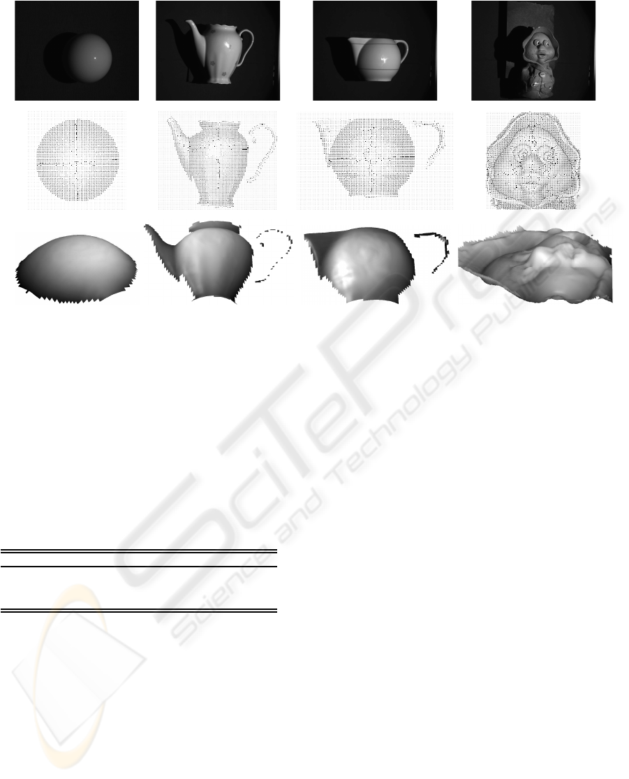
Ball Teapot 1 Teapot 2 Doll
Input imageNormals3D model
Figure 4: Reconstruction results with some real objects.
very small, except for the maximum difference in
which case the larger values are due mostly to oc-
clusions around the object contour. The observation
that the results obtained by the radiometric and alge-
braic methods are similar is compatible with our pre-
vious observation that for this particular camera/light
placement, the algebraic constraint is a good approx-
imation of the radiometric constraint.
Table 1: Angular differences between the normals com-
puted with radiometric and unnormalised algebraic meth-
ods. The values are in degrees.
Ball Teapot 1 Teapot 2 Doll
RMS 0.0219 0.997 1.12 1.87
median 0.0104 0.0077 0.0086 0.0306
max 0.226 25.0 37.8 63.5
5 CONCLUSIONS
In this paper, we proposed a novel method for surface
normal reconstruction using HS. The method is based
on the minimisation of a cost function which consists
of squared radiometric distances summed over all re-
ciprocal pairs of images in which a surface point is
visible. Physically, the cost function represents the
modification to be applied to the intensities of the
projected surface point in order to satisfy exactly the
Helmholtz reciprocity principle. The normal com-
puted by this method has been shown to be an ML
estimate under standard Gaussian noise assumption.
A solution can be computed at low computational cost
due to the low number of optimisation variables.
In the case of synthetic data, it was verified exper-
imentally that the method based on the radiometric
distance results in more accurate surface normal esti-
mates than methods based on SVD. Experiments car-
ried out with real imagery showed that the proposed
method produces similar results to SVD-based meth-
ods for the experimentalset-up considered, and is able
to generate realistic 3D models for a variety of objects
with challenging surface properties.
In future work, we would like to build a more ver-
satile experimental set-up which would allow more
freedom in camera/light source placement, by e.g.
mounting a pair of camera/light source on a robot
arm. Such a set-up would allow reconstruction of a
full 3D model instead of the current 2.5D representa-
tion. In this scenario, we would also expect larger dif-
ferences in performance between the algebraic meth-
ods and the radiometric method, and we may be able
to measure the optimality of the radiometric method
under real noise conditions.
ACKNOWLEDGEMENTS
The authors would like to acknowledge the sup-
port of EPSRC project GR/R08629/01, EU project
MRTN-CT-2004-005439 Visiontrain, and the Czech
Academy of Sciences project 1ET101210406.
VISAPP 2008 - International Conference on Computer Vision Theory and Applications
358

REFERENCES
Cook, R. L. and Torrance, K. E. (1982). A reflectance model
for computer graphics. ACM Transactions on Graph-
ics, 1(1):7–24.
Guillemaut, J.-Y., Drbohlav, O.,
ˇ
S´ara, R., and Illingworth,
J. (2004). Helmholtz stereopsis on rough and strongly
textured surfaces. In Proc. International Symposium
on 3D Data Processing, Visualization and Transmis-
sion, pages 10–17.
Hartley, R. I. (1997). In defence of the eight-point algo-
rithm. IEEE Transactions on Pattern Analysis and
Machine Intelligence, 19(6):580–593.
Jank´o, Z., Drbohlav, O., and
ˇ
S´ara, R. (2004). Radiometric
calibration of a Helmholtz stereo rig. In Proc. IEEE
Conference on Computer Vision and Pattern Recogni-
tion, volume 1, pages 166–171.
Lafortune, E. P. and Willems, Y. D. (1994). Using the modi-
fied phong reflectance model for physically based ren-
dering. Technical Report CW 197, Department of
Computing Science, K.U. Leuven, November, 1994.
Lewis, R. R. (1994). Making shaders more physically plau-
sible. Computer Graphics Forum, 13(2):109–120.
Magda, S., Kriegman, D. J., Zickler, T., and Belhumeur,
P. N. (2001). Beyond Lambert: Reconstructing sur-
faces with arbitrary BRDFs. In Proc. IEEE Inter-
national Conference on Computer Vision, volume 2,
pages 391–398.
Nicodemus, F. E., Richmond, J. C., Hsia, J. J., Ginsberg,
I. W., and Limperis, T. (1977). Geometrical consider-
ation and nomenclature for reflectance. NBS Mono-
graph 160.
Press, W. H., Teukolsky, S. A., Vetterling, W. T., and Flan-
nery, B. P. (1992). Numerical recipes in C. Cambridge
University Press, second edition.
Sen, P., Chen, B., Garg, G., Marschner, S. R., Horowitz,
M., Levoy, M., and Lensch, H. P. A. (2005). Dual
photography. ACM SIGGRAPH, 24(3):745–755.
Terzopoulos, D. (1982). Multi-level reconstruction of visual
surfaces: Variational principles and finite element rep-
resentations. A.I. Memo 671, MIT.
Tu, P. and Mendonc¸a, P. R. S. (2003). Surface reconstruc-
tion via Helmholtz reciprocity with a single image
pair. In Proc. IEEE Conference on Computer Vision
and Pattern Recognition, volume 1, pages 541–547.
Tu, P., Mendonc¸a, P. R. S., Ross, J., and Miller, J. (2003).
Surface registration with a Helmholtz reciprocity im-
age pair. In IEEE Workshop on Color and Photometric
Methods in Computer Vision.
Zickler, T. (2006). Reciprocal image features for uncali-
brated helmholtz stereopsis. In Proc. IEEE Confer-
ence on Computer Vision and Pattern Recognition,
volume 2, pages 1801–1808.
Zickler, T., Belhumeur, P. N., and Kriegman, D. J. (2002a).
Helmholtz stereopsis: Exploiting reciprocity for sur-
face reconstruction. In Proc. European Conference on
Computer Vision, volume III, pages 869–884.
Zickler, T. E., Belhumeur, P. N., and Kriegman, D. J.
(2002b). Helmholtz stereopsis: Exploiting reciprocity
for surface reconstruction. International Journal of
Computer Vision, 49(2/3):215–227.
Zickler, T. E., Belhumeur, P. N., and Kriegman, D. J.
(2003a). Toward a stratification of Helmholtz stere-
opsis. In Proc. IEEE Conference on Computer Vision
and Pattern Recognition, volume 1, pages 548–555.
Zickler, T. E., Ho, J., Kriegman, D. J., Ponce, J., and Bel-
humeur, P. N. (2003b). Binocular Helmholtz stereop-
sis. In Proc. IEEE International Conference on Com-
puter Vision, pages 1411–1417.
APPENDIX
Simplification of the Cost Function based
on the Radiometric Distance
We would like to compute the values n and {
ˆ
i
l
j
}
j
which minimise the cost function F defined by:
F(n, {
ˆ
i
l
j
}
j
) =
∑
j
[(
ˆ
i
l
j
−i
l
j
)
2
+(
s
l
j
· n
s
r
j
· n
ˆ
i
l
j
−i
r
j
)
2
]. (18)
We start by writing the partial derivatives of F with
respect to
ˆ
i
l
k
; for any index k in {1, . . . , N}, we have:
∂F(n, {
ˆ
i
l
j
}
j
)
∂
ˆ
i
l
k
= 2(
ˆ
i
l
k
− i
l
k
) + 2
s
l
k
· n
s
r
k
· n
(
s
l
k
· n
s
r
k
· n
ˆ
i
l
k
− i
r
k
).
(19)
At the optimum, the partial derivatives must be zero;
this results in the following constraints:
∀k,
ˆ
i
l
k
+ (
s
l
k
· n
s
r
k
· n
)
2
ˆ
i
l
k
= i
l
k
+
s
l
k
· n
s
r
k
· n
i
r
k
, (20)
from which, we can deduce that, at the optimum, the
values of the variables
ˆ
i
l
k
are:
∀k,
ˆ
i
l
k
=
i
l
k
(s
r
k
· n)
2
+ i
r
k
(s
l
k
· n)(s
r
k
· n)
(s
l
k
· n)
2
+ (s
r
k
· n)
2
. (21)
After substitution of these values into Eq. (18), we
obtain the simplified cost function G defined by:
G(n) =
∑
j
[(i
l
j
s
l
j
− i
r
j
s
r
j
) · n]
2
(s
l
j
· n)
2
+ (s
r
j
· n)
2
. (22)
G defines a simpler cost function with single unknown
n (two degrees of freedom) which has the same global
minimum as the original cost function F.
A MAXIMUM LIKELIHOOD SURFACE NORMAL ESTIMATION ALGORITHM FOR HELMHOLTZ STEREOPSIS
359
