LUCAS-KANADE INVERSE COMPOSITIONAL USING

MULTIPLE BRIGHTNESS AND GRADIENT CONSTRAINTS

Ahmed Fahad and Tim Morris

School of Computer Science, The University of Manchester, Kilburn Building, Oxford Road,Manchester, M13 9PL, UK

Keywords: Lucas-Kanade, Inverse compositional, Motion, Warping.

Abstract: A recently proposed fast image alignment algorithm is the inverse compositional algorithm based on Lucas-

Kanade. In this paper, we present an overview of different brightness and gradient constraints used with the

inverse compositional algorithm. We also propose an efficient and robust data constraint for the estimation

of global motion from image sequences. The constraint combines brightness and gradient constraints under

multiple quadratic errors. The method can accommodate various motion models. We concentrate on the

global efficiency of the constraint in capturing the global motion for image alignment. We have applied the

algorithm to various test sequences with ground truth. From the experimental results we conclude that the

new constraint provides reduced motion error at the expense of extra computations.

1 INTRODUCTION

Since the problem of motion computation is under-

constrained, additional constraints are required for

the estimation techniques. Techniques for estimating

2D camera motion constrain the motion explicitly by

parameterization of the camera motion over the

whole image using different motion models

(translational, affine, pseudo projective, projective).

In numerous dynamic scene analysis and video

compression methods, it is useful to first recover the

camera motion and then to detect and track moving

objects in the scene. Parameter motion estimation

methods can be classified into three categories:

 Error minimization with respect to motion

parameters using differential methods.

 Error minimization with respect to motion

parameters using matching techniques.

 Two-step methods consisting of local motion

estimation followed by global motion

estimation.

A comprehensive comparative survey by Barron

et al. (Barron et al., 1994) found that gradient-based

motion estimation methods (GMs) to perform well

especially Lucas-Kanade (Lucas and Kanade, 1981).

The usual approach of Lucas-Kanade is a gradient

descent approach to estimate the parameters vector p

associated with the parametric image registration. It

aligns a template image T(x) to an input image I(x),

where x=(x,y) is a column vector of pixel

coordinates. The method searches for the best

parametric transform that minimizes the summed

square of differences between image intensities

(SSD) over the whole image by an additive

increment to the motion parameters. Other

approaches estimate an incremental warp that is

composed with the current parameter estimate

(Baker and Matthews, 2004). Minimizing the SSD

error using the Gradient descent approach (non-

linear optimization) requires the partial derivatives

of the equation with respect to ∆p, which involves

computing the inverse of the Hessian matrix that

depends on the parameters p. The Hessian must be

re-evaluated at each iteration of the Lucas-Kanade

algorithm at a huge computational cost, but if the

Hessian is constant it could be precomputed and

reused. The Hager-Belhumeur algorithm (Hager and

Belhumeur, 1998) addresses this difficulty by

switching the role of the template and the image

producing a Hessian that is independent of p. Baker

and Matthews (Baker and Matthews, 2004) also

switch the roles of the template and image but used

composition to update the warps and called their

algorithm the inverse compositional. The advantage

of the inverse compositional algorithm is that it can

be applied to any set of warps. Other approaches

propose to address divergence problems of the

iterative warping nature of Lucas-Kanade (Le

565

Fahad A. and Morris T. (2008).

LUCAS-KANADE INVERSE COMPOSITIONAL USING MULTIPLE BRIGHTNESS AND GRADIENT CONSTRAINTS.

In Proceedings of the Third International Conference on Computer Vision Theory and Applications, pages 565-570

DOI: 10.5220/0001083405650570

 SciTePress

Besnerais and Champagnat, 2005). Other

computational reduction approaches use a sampled

set of pixels for parameter estimation and avoid

computing interpolation at each iteration (Keller and

Averbuch, 2003). In (Keller and Averbuch, 2004) a

bidirectional formulation is introduced that speeds

up the convergence properties for large motions.

Recently, Thomas et al. (Brox et al., 2004),

introduced a robust method to compute the optical

flow by adding to the brightness data constraint of

the energy functional another constraint: the gradient

constraint. The new energy functional produced one

of the best optical flow results in the current

literature. Therefore, a comparison is needed to

show the benefits of combining the gradient

constraint with the brightness constraint for

estimating the global motion.

Over-constraining the optical flow problem allows

more precise determination of a solution. The use of

redundant information enforces robustness with

respect to measurement noise. Constraints can be

obtained using several approaches by either applying

the same equation to multiple points or defining

multiple constraints for each image point. The later

can be obtained by applying a set of differential

equations (Bimbo et al., 1996) or applying the same

set of equations to different functions which are

related to image brightness. When the image motion

conforms to the model assumptions it produces

accurate flow estimates. However, the problem is

that parametric motion models applied over the

entire image are rarely valid due to varying depths,

transparency or independent motion. Therefore, It is

useful to use robust statistics to estimate a dominant

motion in the scene and then fit additional motions

to outlying measurements (Black and Jepson, 1996,

Irani et al., 1994). The outlying measurements which

are grouped together and segmented correspond to

independently moving objects and their motion is

estimated independently. It is also well-known that

the use of multiresolution methods improves the

estimation for large motions (Odobez and

Bouthemy, 1995). Spatiotemporal information gives

better results than spatial information (Barron et al.,

1994), and specifically, spatiotemporal

neighbourhood information assists in obtaining

better estimates for the motion vectors (Namuduri,

2004).

In this paper, we begin in section 2 by reviewing

the inverse compositional Lucas-Kanade algorithm

using only the brightness constancy. We proceed in

section 3 to elaborate on the constancy assumptions

by using the gradient constancy alone or combined

with the brightness constancy. In section 4 we

propose a new data constraint that combines the

brightness constancy with the gradient constancy

using multiple quadratic error functions. We

compare empirically the different data constraints in

section 5 both in terms of performance and speed.

We conclude in section 6.

2 INVERSE COMPOSITIONAL

IMAGE ALIGNMENT

Let W(x,p) denote a warping function that takes the

pixel x and maps it to subpixel location W(x,p)

where p=(p

,..,p

)

is a vector of motion parameters.

The goal of the inverse compositional (Baker and

Matthews, 2004) is to align a template image T(x) to

an input image I(x), where x=(x,y)

is a vector of

pixel coordinates. The inverse compositional

minimizes the sum of the squared differences (SSD)

between the current frame T and the motion

compensated frame I

() ( (; )) ( (;))

Ep TWxpIWxp=Δ−

⎡

⎤

⎣

⎦

∑

(1)

with respect to ∆p, where ∆p is the incremental

update to the motion parameters p by updating the

warp:

(;) (;) (; )Wxp Wxp Wx p

−

←Δo

(2)

Computing the backward warp of the image

I(W(x;p)) requires interpolating the image at

subpixel locations. Before deriving the solution, a

first order Taylor expansion is performed on (1):

((;0)) ((;))

TW x T p IW x p

⎡

⎤

∂

+∇ Δ −

⎢

⎥

∂

⎣

⎦

∑

(3)

where W(x;0) is the identity warp. Solving the least

squares equation for ∆p gives:

((;) ()

pH T IWxpTx

−

⎡⎤

∂

Δ= ∇ −

⎡

⎤

⎢⎥

⎣

⎦

∂

⎣⎦

∑

(4)

where H is the Hessian matrix:

HT T

⎡

⎤⎡ ⎤

∂∂

=∇ ∇

⎢

⎥⎢ ⎥

∂∂

⎣

⎦⎣ ⎦

∑

(5)

Assuming affine warp p=(p1,p2,p3,p4,p5,p6),

135

246

(;)

ppp

Wxp y

ppp

⎛⎞

⎜⎟

⎝⎠

⎜⎟

⎝⎠

(6)

VISAPP 2008 - International Conference on Computer Vision Theory and Applications

566

and the Jacobian of the warp

/Wp∂∂

is then:

0010

0001

xx x

yy y

WW W

pp p

WW W

pp p

∂∂ ∂

⎛⎞

⎜⎟

⎛⎞

⎜⎟

⎝⎠

⎜⎟

⎝⎠

(7)

The inverse compositional algorithm using the

brightness constancy (BC) then consists of

iteratively applying (4) and (2). In Summary:

Precompute:

(1) Evaluate the gradient

T∇

of the template T(x)

(2) Evaluate the Jacobian

/Wp∂∂at (x;0)

(3) Compute the steepest descent images

(/)TW p∇∂ ∂

(4) Compute the Hessian matrix using (5).

Iterate:

(5) Warp I with W(x;p) to compute I(W(x;p))

(6) Compute the error image I(W(x;p))-T(x)

(7) Compute

((;) ()

TIWxpTx

⎡⎤

∂

∇−

⎡⎤

⎢⎥

⎣⎦

∂

⎣⎦

∑

(8) Compute ∆p using (4)

(9) Update the warp using (2)

Until ||∆p||≤ε.

3 VARIANT CONSTANCY

ASSUMPTIONS

Although the brightness constancy (BC) assumption

works well, it cannot deal with either local or global

changes in illumination. Other constancy

assumptions such as the gradient constancy

assumption (which assumes the spatial gradients of

an image sequence to be constant during motion) are

applied. A global change in illumination affects the

brightness values of an image by either shifting or

scaling or both. Shifting the brightness will not

change the gradient; scaling affects the magnitude of

the gradient vector but not its direction.

The inverse compositional using the gradient

constancy (GC) minimizes the sum of the squared

differences (SSD) between the gradient of the

current frame

T∇

and the gradient of motion

compensated frame

I∇

() ( (; )) ( (;))

Ep TWxp IWxp∇Δ−∇

⎡⎤

⎣⎦

∑

(8)

with respect to to ∆p then updates the warp using

(2). Performing a first order Taylor expansion:

((;0)) ( ) ((;))

TW x T p IW x p

⎡

⎤

∂

∇+∇∇Δ−∇

⎢

⎥

∂

⎣

⎦

∑

(9)

Solving the least squares equation for ∆p gives:

() ((;) ()

HTIWxpTx

−

⎡⎤

∂

Δ= ∇∇ ∇ −∇

⎡⎤

⎢⎥

⎣⎦

∂

⎣⎦

∑

(10)

where H is the Hessian matrix:

() ()

HT T

⎡

⎤⎡ ⎤

∂∂

=∇∇ ∇∇

⎢

⎥⎢ ⎥

∂∂

⎣

⎦⎣ ⎦

∑

(11)

The GC inverse compositional algorithm using the

gradient constraint then consists of iteratively

applying (10) and (2).

Not all constancy assumptions based on

derivatives perform equally well, neither are they

well-suited to estimate different types of motion.

Over-constraining the problem and using redundant

information allows for estimation robust against

noise. Using the brightness constraint and the

gradient constraint in the inverse compositional (BC

GC) minimizes the sum of the squared differences

(SSD) between the current frame T and the motion

compensated frame I and also minimizes the sum of

the squared differences (SSD) between the gradient

of the current frame

∇

and the gradient of motion

compensated frame

∇

(

)

() ( (; )) ( (;))

((; )) ((;))

BC GC

EpTWxpIWxp

TW x p IW x p

Δ− +

⎡⎤

⎣⎦

∇Δ−∇

⎡

⎤

⎣

⎦

∑

(12)

with respect to ∆p then updates the warp using (2).

Performing a first order Taylor expansion and

solving the least squares equation for ∆p gives:

((;) ()

() ((;) ()

pH T IWxpTx

HTIWxpTx

−

⎡⎤

∂

Δ= ∇ − +

⎡⎤

⎢⎥

⎣⎦

∂

⎣⎦

⎡⎤

∂

∇∇ ∇ −∇

⎡⎤

⎢⎥

⎣⎦

∂

⎣⎦

∑

(13)

where H is the Hessian matrix:

() ()

HT T

⎡⎤⎡⎤

∂∂

=∇ ∇ +

⎢⎥⎢⎥

∂∂

⎣⎦⎣⎦

⎡

⎤⎡ ⎤

∂∂

∇∇ ∇∇

⎢

⎥⎢ ⎥

∂∂

⎣

⎦⎣ ⎦

∑

(14)

LUCAS-KANADE INVERSE COMPOSITIONAL USING MULTIPLE BRIGHTNESS AND GRADIENT

CONSTRAINTS

567

The BC GC inverse compositional algorithm using

the brightness and gradient constraint then consists

of iteratively applying (13) and (2).

While the previous approach allows both the

brightness constraint and the gradient constraint to

compete for minimizing the error, another approach

would combine the brightness and the gradient

constraints using one quadratic error. The combined

inverse compositional (BC+GC) minimizes the sum

of the squared differences (SSD) between the

brightness of the current frame T and the motion

compensated frame I plus the gradient of the current

frame

T∇

and the gradient of motion compensated

frame

I∇

()

() ( (; )) ( (;))

((; )) ((;))

BC GC

EpTWxpIWxp

TW x p IW x p

=Δ−+

⎡

⎣

⎤

∇Δ−∇

⎦

∑

(15)

with respect to ∆p then updates the warp using (2). γ

is a balancing constant. Performing a first order

Taylor expansion and solving the least squares

equation for ∆p gives:

()

() ((;)

() ( (;) ()

pH T T IWxp

Tx IWxp Tx

−

⎡⎤

∂

Δ= ∇ +∇∇ −

⎡⎤⎡

⎢⎥

⎣⎦⎣

∂

⎣⎦

⎤

+∇ −∇

⎦

∑

(16)

where H is the Hessian matrix:

() ()

HTT TT

γγ

⎡⎤⎡⎤

∂∂

= ∇ +∇∇ ∇ +∇∇

⎡⎤⎡⎤

⎢⎥⎢⎥

⎣⎦⎣⎦

∂∂

⎣⎦⎣⎦

∑

(17)

The BC+GC inverse compositional algorithm using

the combined brightness and gradient constraint then

consists of iteratively applying (16) and (2).

4 MULTIPLE COMBINED

BRIGHTNESS AND GRADIENT

CONSTRAINTS

The previous data constraints produced different

results for each frame and some data constraints

achieved better results for some frames while failing

to compete at other frames. Therefore, a better data

constraint would exploit the advantages of each data

constraint in a combined constraint to yield better

results. Consequently, we propose to combine the

brightness constraint combined with the gradient

constraint in equation (15) to compete with the

gradient constraint in equation (8). The new

proposed constraint multiple combined (CBG)

achieved better results over all sequences applied

when compared to ground truth. The new inverse

compositional algorithm minimizes the sum of the

squared differences (SSD) between the brightness T

and the gradient

∇

of the current frame and the

motion compensated frame I and its gradient

∇

and also minimizes the sum of the squared

differences between the gradient

T∇

and the motion

compensated frame gradient

I∇

()

() ( (; )) ( (;))

((; )) ((;))

CBG

Ep TWxpIWxp

TW x p IW x p

=Δ−+

⎡

⎣

⎤

∇

Δ−∇ +

⎦

∇Δ−∇

⎡

⎤

⎣

⎦

∑

(18)

with respect to ∆p then updates the warp using (2).

Performing a first order Taylor expansion solving

the least squares equation for ∆p gives:

[][

()

[]

() () ((;)

() ( (;) ()

()() ((;)()

pHH T T IWxp

Tx IWxp Tx

HH T IWxp Tx

−

∂

=+ ∇+∇∇ −

∂

∇−∇+

∂

+∇∇∇−∇

∂

⎡⎤

⎢⎥

⎣⎦

⎤

⎦

⎡⎤

⎢⎥

⎣⎦

∑

(19)

where H1 and H2 are:

() ()

HTT TT

γγ

⎡

⎤⎡ ⎤

∂∂

=∇+∇∇ ∇+∇∇

⎡⎤⎡⎤

⎢

⎥⎢ ⎥

⎣⎦⎣⎦

∂∂

⎣

⎦⎣ ⎦

∑

() ()

HT T

⎡

⎤⎡ ⎤

∂∂

=∇∇ ∇∇

⎢

⎥⎢ ⎥

∂∂

⎣

⎦⎣ ⎦

∑

(20)

The CBG inverse compositional algorithm using the

multiple combined brightness and gradient

constraint then consists of iteratively applying (19)

and (2).

5 EXPERIMENTS

We performed our experiments on three synthetic

image sequences that have ground truth: Yosemite

sequence, Office sequence and Street sequence

(www.katipo.otago.ac.nz/research/vision/). The

algorithms have been implemented in Matlab on a

1.5 GHz Intel Centrino. The moving objects

VISAPP 2008 - International Conference on Computer Vision Theory and Applications

568

considered are the sky in the Yosemite sequence, the

car in the Street sequence. The Office sequence does

not have any moving objects. The balancing factor

between the brightness and gradient γ is fixed for all

sequences and all equations at 5 or 10. All the

algorithms require between 10 and 25 iterations to

converge. Most importantly, the algorithms all

converge equally fast. We only include the results

using the affine motion. In this experiment we

estimate the global motion of each scene using the

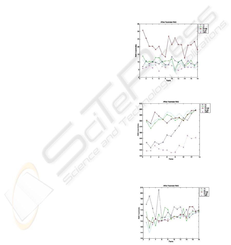
five data constraints. Figure 1 shows the mean

square error between the estimated global motion

and the correct one using the five data constraints. A

direct comparison between the angular errors of the

method using the multiple combined constraints and

the other constraints respectively, quantifies the

improvement achieved with our technique. The

Iterative reweighted least squares method is

sufficient to reject outliers because the moving

objects are small compared to the global motion in

each sequence. Figures 1,2 and 3 shows that our

method is globally the best compared to other

approaches, however other constraints perform

better in some frames. Therefore, in the future, we

intend to investigate different robust functions that

respect occlusion and other anomalies.

Table 1 shows a comparison of the average

angular error (AAE) of the estimated flow compared

to the correct motion for each sequence using the

five data constraints. The results are only for affine

warp. The first thing to notice in Table 1 is that the

best performing data constraint is the Multiple

combined CBG. The second thing to notice is that

the brightness constraint performs fairly compared

to other constraints. In general, we expect the

multiple combined data constraint to perform better

because it uses a more sophisticated estimate of the

Hessian. That expectation, however, relies on the

assumption that the estimate of the Hessian is

noiseless.

In the next experiment we tested our data

constraints on a real sequence. The sequence

represents zooming by a walking person.

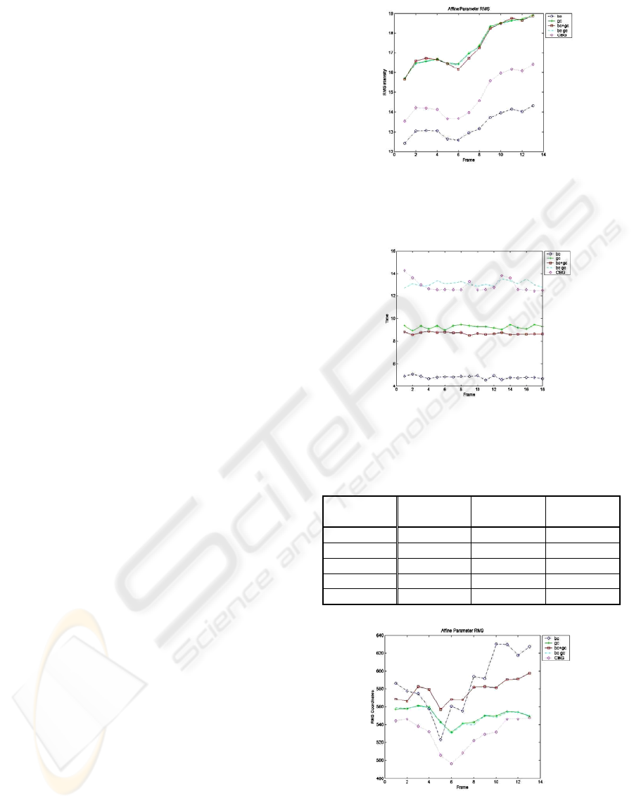
Effectively, the brightness constraint gives the

lowest mean intensity error among all other

approaches. However, this small error does not

reflect better estimation. Figure 4 shows the RMS

intensity error for the Yosemite sequence with the

BC having the smallest intensity error.

Figure 5 shows the average time taken when

processing each data constraint and we notice that

our new data constraint is more complicated and

requires more computation compared to the simple

brightness constraint. This trade off between quality

and time favours the brightness constraint.

In the last experiment, we test the data constraints

using different robust approximations to the inverse

compositional algorithm. Dividing the frame into

blocks and estimating the Hessian on each block of

pixels allows for a robust inverse compositional

without iterative computation to the Hessian. The

final Hessian equals the sum of all block Hessians

then the motion parameters are estimated. This local

estimation to the Hessian reflects the strength of the

data constraint globally. Figure 6 shows the result on

the Yosemite sequence.

Figure 1: Street sequence average RMS coordinates error.

Figure 2: Yosemite sequence average RMS coordinates

error.

Figure 3: Office sequence average RMS coordinates error.

LUCAS-KANADE INVERSE COMPOSITIONAL USING MULTIPLE BRIGHTNESS AND GRADIENT

CONSTRAINTS

569

6 CONCLUSIONS

We have described two data constraints for image

alignment using the inverse compositional

algorithm. When applied to synthesized image

sequences, the method is capable of delivering

smaller error rates compared to known data

constraints.

REFERENCES

Baker, S. and I. Matthews (2004). Lucas-Kanade 20 Years

On: A Unifying Framework. International J. of

Computer Vision 56(3): 221-255.

Barron, J. L., D. J. Fleet, et al. (1994). Performance of

Optical Flow Techniques. International J. of

Computer Vision, 12(1): 43-77.

Bimbo, A. D., P. Nesi, et al. (1996). Optical Flow

Computation Using Extended Constraints. IEEE

Trans. on Image Processing 5(5): 720-732.

Black, M. J. and A. Jepson (1996). Estimating Optical

Flow in Segmented Images using Variable-order

Parametric Models with Local Deformations. IEEE

Trans on PAMI, 18(10): 972 - 986.

Brox, T., A. e. Bruhn, et al. (2004). High Accuracy

Optical Flow Estimation Based on a Theory for

Warping. 8th European Conf. on Computer Vision.

Springer.

Hager, G. D. and P. N. Belhumeur (1998). Efficient region

tracking with parametric models of geometry and

illumination. IEEE Trans. PAMI, 20(10): 1025-1039.

Irani, M., B. Rousso, et al. (1994). Computing Occluding

and Transparent Motions. International Journal of

Computer Vision 12(1): 5-16.

Keller, Y. and A. Averbuch (2003). Fast Gradient

Methods Based on Global Motion Estimation for

Video Compression. IEEE Transactions on circuits

and systems for video technology 13(4): 300-309.

Keller, Y. and A. Averbuch (2004). Fast Motion

Estimation Using Bidirectional Gradient Methods.

IEEE Trans. on Image Processing 13(8): 1042-1052.

Le Besnerais, G. and F. Champagnat (2005). Dense optical

flow by iterative local window registration. IEEE

International Conference on Image Processing.

Lucas, B. D. and T. Kanade (1981). An Iterative Image

Registration Technique with an Application to Stereo

Vision. Proceedings of Seventh International Joint

Conference on Artificial Intelligence, Canada.

Namuduri, K. R. (2004). Motion estimation using spatio-

temporal contextual information. IEEE Trans. on

circuits systems for video technology 14(8): 1111-

1115.

Odobez, J. M. and P. Bouthemy (1995). Robust

Multiresolution estimation of parametric motion

models. Inter. J. of Visual Communication and Image

Representation 6(4): 348-365.

Figure 4: Yosemite sequence average RMS intensity error.

The small intensity error for the BC data constraint does

not reflect correct motion compared to ground truth.

Figure 5: Timing results computed for each data

constraint.

Table 1: RMS mean error for the five data constraints

applied to street, yosemite and office sequence.

Average

RMS for

Street Yosemite Office

BC 9.59 561.97 169.64

GC 10.14 584.34 159.99

BC+GC 20.96 586.14 158.69

BC_GC 8.18 588.66 155.88

CBG 6.48 535.92 156.34

Figure 6: Yosemite sequence average RMS coordinates

error by local estimation of the Hessian on each block.

VISAPP 2008 - International Conference on Computer Vision Theory and Applications

570