VIEW-BASED ROBOT LOCALIZATION USING

ILLUMINATION-INVARIANT SPHERICAL HARMONICS

DESCRIPTORS

Holger Friedrich, David Dederscheck, Martin Mutz and Rudolf Mester

Visual Sensorics and Information Processing Lab, J. W. Goethe University

Robert-Mayer-Str 10, Frankfurt, Germany

Keywords:

Robot localization, spherical harmonics, illumination invariance.

Abstract:

In this work we present a view-based approach for robot self-localization using a hemispherical camera system.

We use view descriptors that are based upon Spherical Harmonics as orthonormal basis functions on the

sphere. The resulting compact representation of the image signal enables us to efﬁciently compare the views

taken at different locations. With the view descriptors stored in a database, we compute a similarity map for

the current view by means of a suitable distance metric. Advanced statistical models based upon principal

component analysis introduced to that metric allows to deal with severe illumination changes, extending our

method to real-world applications.

1 INTRODUCTION

For the purpose of robot localization, omnidirec-

tional vision has become popular during the last

years. Many approaches rely on compact view de-

scriptors (Pajdla and Hlavac, 1999; Blaer and Allen,

2002; Gonzalez-Barbosa and Lacroix, 2002; Levin

and Szeliski, 2004), (Kr

ose et al., 2001; Jogan and

Leonardis, 2003) (using principal component analy-

sis) (Menegatti et al., 2003; Menegatti et al., 2004)

(using Fourier descriptors), (Labbani-Igbida et al.,

2006) (using Haar integrals) to store and compare

views efﬁciently.

We present a view-based method for robot local-

ization in a known environment represented by a set of

reference views. The contribution shown in this paper

is an extension of our previous work (Friedrich et al.,

2007) to more realistic image data. Using real images

imposes various challenges: First, we have to take

care of varying illumination. Second, for practical

reasons an interpolation method for reference views

had to be developed.

A mobile robot equipped with an omnidirectional

camera system provides a spherical image signal

s(θ,φ), i. e. an image signal deﬁned on a sphere. In

our setup, omnidirectional views are obtained from

usual planar images taken by an upward-facing cam-

era, which are subsequently projected onto a semi-

sphere. These images are converted into view descrip-

tors, i. e. low dimensional vectors (Fig. 1), by an ex-

pansion in orthonormal basis functions. The robot lo-

calization task is performed by comparing the current

view descriptor to those stored in a map of the known

environment, i. e. a database of views (Fig. 2).

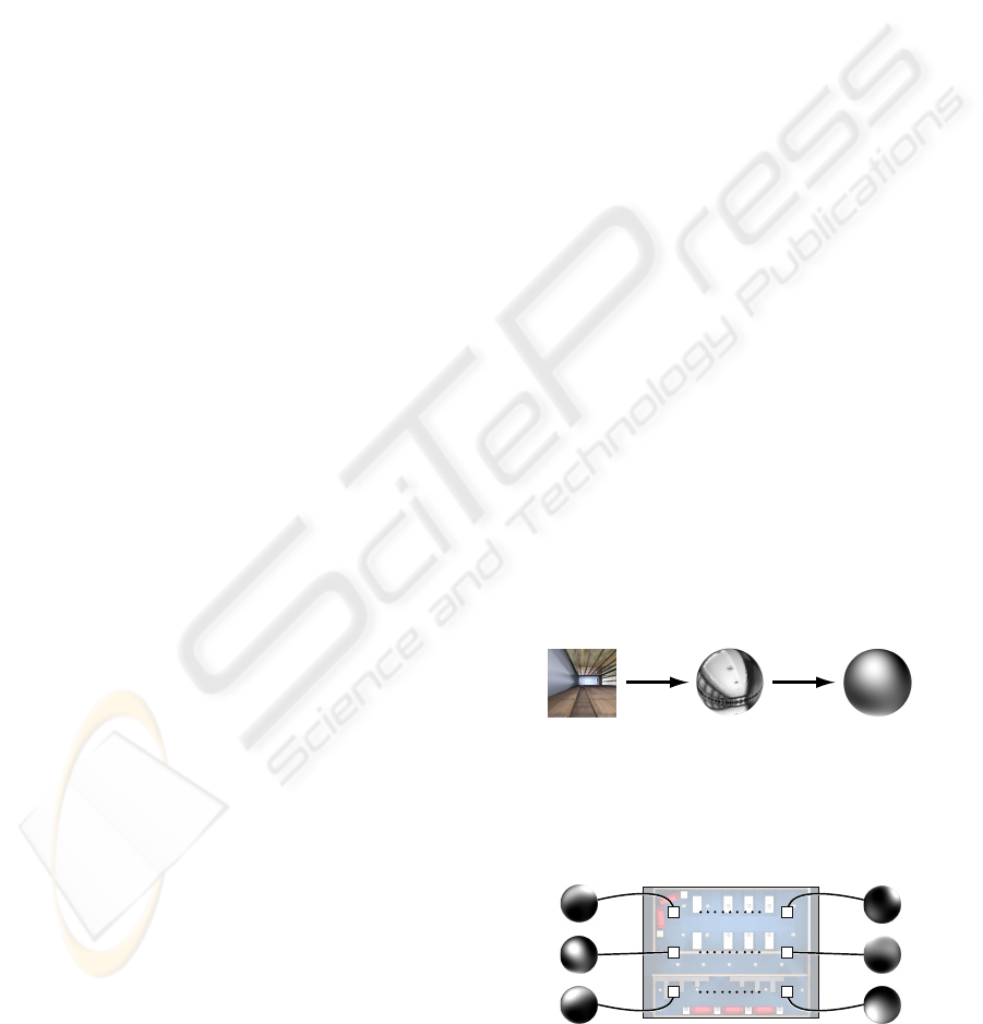
Figure 1: Computing an omnidirectional image signal from

a planar wide angle image. The right image visualizes a low

order Spherical Harmonics descriptor that approximates the

omnidirectional image signal.

Figure 2: A known environment is represented by a map

containing view descriptors. These are obtained from im-

ages taken at reference positions.

543

Friedrich H., Dederscheck D., Mutz M. and Mester R. (2008).

VIEW-BASED ROBOT LOCALIZATION USING ILLUMINATION-INVARIANT SPHERICAL HARMONICS DESCRIPTORS.

In Proceedings of the Third International Conference on Computer Vision Theory and Applications, pages 543-550

DOI: 10.5220/0001083705430550

 SciTePress

Given a suitable distance metric, for each in-

put view taken at an initially unknown robot posi-

tion and orientation, a ﬁgure of (dis-)similarity to

any view stored in the database can be generated di-

rectly from the compact vector representation of these

views. The resulting likelihood of the robot location/-

pose allows for more sophisticated sequential self-

localization strategies (Thrun et al., 2005), e. g. using

particle ﬁlters.

2 VIEW DESCRIPTORS

Our view representation is obtained by expanding the

spherical image signal s(θ,φ) in orthonormal basis

functions. The natural choice for spherical basis func-

tions are Spherical Harmonics (SH) (Fig. 3). Our ap-

proach particularly beneﬁts from using SH since they

show the same nice properties concerning rotations

which the Fourier basis system provides with respect

to translations. Rotations are mapped into a kind of

generalized phase changes.

Spherical Harmonics (SH). Here, we give a very

brief introduction to SH. For group theoretical facts

see (Makadia and Daniilidis, 2006) and (Groemer,

1996), for more details on our notation see (Friedrich

et al., 2007). Let N

2`+1

(`−|m|)!

(`+|m|)!

, ` ∈ N

, m ∈

Z and P

(x) the Associated Legendre Polynomials

(Weisstein, 2007). The SH Y

(θ,φ) are deﬁned as

(θ,φ) =

√

2π

·N

·P

(cosθ) ·e

imφ

(1)

with e

imφ

being a complex-valued phase term. ` (` >

0) is called order and m (m = −`..+`) is called quan-

tum number for each `. SH have several properties

which we exploit in the following sections: Each set

of SH of order ` forms a closed orthonormal basis of

dimension 2` + 1; SH of orders 0...` form a closed

orthonormal basis of dimension (` + 1)

, hence

2π

(θ,φ) ·Y

(θ,φ) ·sin θ dθ dφ = δ

·δ

(2)

where δ

is the Kronecker delta function.

3 DoF rotation. Since SH of order ` and of order

0...` form a closed basis, any 3D rotation can be ex-

pressed as a linear transformation (i. e. multiplication

with an unitary matrix U

for each order `) and does

not mix coefﬁcients of different orders. Hence rota-

tions retain the distribution of spectral energy among

different orders (Makadia and Daniilidis, 2006; Kazh-

dan et al., 2003). This is a unique characteristic of

SH which makes them so particularly useful, amongst

others for the purpose of robot ego-localization pur-

sued here. Applying a 3D rotation to a spherical func-

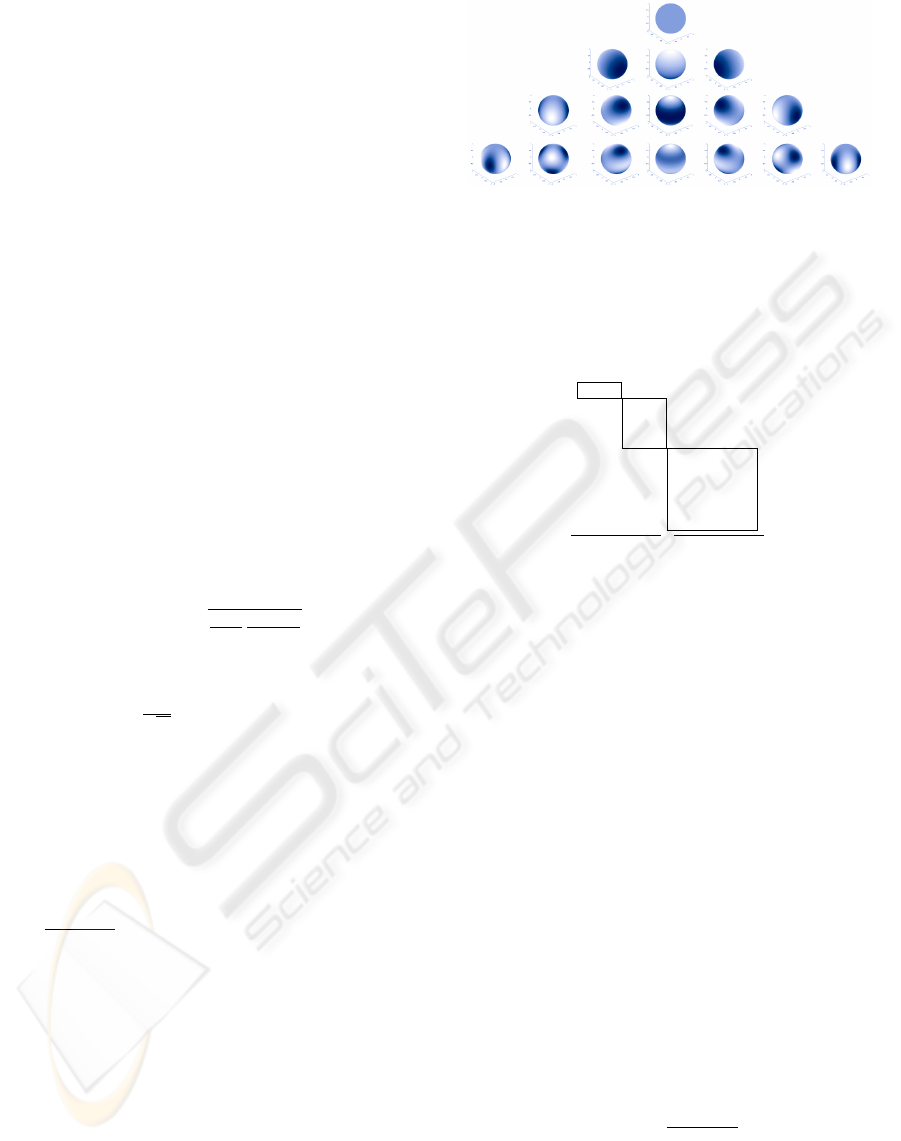
Figure 3: A Spherical Harmonics function is a periodic

function on the unit sphere. The rows show SH of orders.

` = 0,1,2,3; columns show m = 2` + 1 functions for each

order `.

tion represented by coefﬁcients a

yields new coefﬁ-

cients b

according to







1,−1

2,−2













`=0

`=1

0 U

`=2







{z }

tot







1,−1

2,−2







(3)

Rotation estimation has been treated by (Burel and

Henoco, 1995), and more recently in (Makadia, 2006;

Makadia and Daniilidis, 2006; Makadia and Dani-

ilidis, 2003; Kovacs and Wriggers, 2002).

1 DoF rotation about X

-axis. As an initial test case,

we have chosen a mobile robot moving on a plane.

For this particular application we only need to deal

with 1D rotation estimation. Recalling the deﬁnition

of the complex-valued SH, the implications of a rota-

tion of ϕ about the X

-axis are as follows:

(θ,φ + ϕ) = e

im ϕ

·Y

(θ,φ). (4)

The rotation matrix changes into a diagonal matrix

with elements e

−imϕ

, thus

= e

−imϕ

·a

. (5)

SH Expansion. To approximate a signal s(θ,φ), i. e.

s(θ,φ) =

∑

∞

`=0

∑

m=−`

·Y

(θ,φ), (6)

the coefﬁcients a

are obtained by computing scalar

products between the signal and the complex conju-

gate of each of the basis functions:

2π

s(θ,φ) ·Y

(θ,φ) ·sin θ dθ dφ. (7)

In practice, this is done using SH of order ` = 0 up

to a small number, e. g. ` = 4, resulting in a notable

compression of the input image to a 25-dimensional

vector.

VISAPP 2008 - International Conference on Computer Vision Theory and Applications

544

3 LOCALIZATION

3.1 Similarity Measure

Similarity between two view descriptors, ~a for signal

g(θ,φ) and

b for signal h(θ, φ), can be deﬁned in a nat-

ural way. We deﬁne the dissimilarity Q as the squared

difference of two image signals in the SH domain up

to order `:

2π

(g(θ,φ) −h(θ, φ))

·sinθ dθdφ

Eq. 6

2π



∑

∞

`=0

∑

m=−`

−b

) ·Y

(θ,φ)



·sinθ dθdφ

Eq. 2

∑

∞

`=0

∑

m=−`

∑

∞

∑

=−`

−b

)

·(a

−b

) ·δ

·δ

= ||~a −

b||

(8)

This result is of course a consequence of the basis sig-

nals forming an orthonormal basis. The measure Q is

sensitive to any rotation between the signals. Hence,

to ﬁnd the minimum dissimilarity of two view de-

scriptors we ﬁrst have to de-rotate them, i. e. compen-

sate for the unknown rotation.

3.2 De-Rotation

Currently our implementation is based on direct non-

linear estimation of ϕ similar to the method described

in (Makadia et al., 2004). In this method, the 3D-

rotation U

tot

for view descriptors ~a and

b is deter-

mined such that ||

b − U

tot

~a||

is minimized. The con-

straint of mere 1-axis rotation, which has been main-

tained in our experiments so far, leads to simpliﬁca-

tions: we have to determine the angle ϕ that mini-

mizes

∑

m=−`

− e

−imϕ

)

. We emphasize

that full 3D de-rotation is possible (Makadia et al.,

2004; Makadia and Daniilidis, 2006) for other robot

conﬁgurations, that is, the SH approach is even more

interesting in that case.

3.3 Rotation Invariant Similarity

As coefﬁcients corresponding to different orders of

SH are not mixed in rotations, the norms of these sub-

groups of coefﬁcients are invariant to arbitrary 3D ro-

tations of the signal. Thus L

norms, one for each

order of SH, can be considered as a kind of energy

spectrum of the omnidirectional signal.

This energy spectrum is an efﬁcient means for

comparing pairs of spherical signals (Kazhdan et al.,

2003). With a proper metric, spherical signals can

be compared to each other even without performing

the de-rotation. Only if the energy spectrum is iden-

tical or similar, the particular spherical signals can be

identical. Hence, the energy spectrum can be used as

a preﬁltering in a matching process.

3.4 Robot Localization Algorithm

We perform the localization task by calculating a dis-

tance measure between the current view descriptor

and each reference location:

1. First, we use the fast rotation invariant similarity

measure to drop all unlikely views.

2. Then, for all reference views which survived this

‘preﬁltering’ we estimate the best matching rota-

tion with respect to the current view descriptor

and de-rotate it accordingly. Thereafter, we com-

pute the similarity according to the measure intro-

duced in Sec. 3.1.

The resulting similarity map typically shows a distinct

extremum at the true location of the robot. As our ex-

periments have shown, there can also be additional

extrema of similar likelihood for different poses. This

corresponds to the regularities of man-made environ-

ments resulting in similar views at more than one

position. At each instant, however, we have prior

knowledge about the previous course of the robot and

its previous pose, which is presumably always suf-

ﬁcient to disambiguate the pose estimation process.

Such strategies are well-known in robot navigation

and have been, amongst many others, described by

Thrun et al. (Thrun et al., 2005) (‘Monte Carlo Local-

ization’), or Menegatti et al. (Menegatti et al., 2003)

(using different view descriptors).

4 ILLUMINATION INVARIANCE

Changes in illumination are an inevitable issue to deal

with in most vision applications (Mester et al., 2001;

Steinbauer and Bischof, 2005). Thus, when perform-

ing localization we need to introduce methods that

disregard the effects by illumination changes on the

measured distance between two view descriptors.

4.1 Multiplicative Illumination Model

The most simple model for illumination changes is

a global multiplicative change, i. e. the brightness of

each pixel in the source image is multiplied by the

same number α. This kind of change can of course be

easily compensated for by normalization. For typical

views at different illumination conditions, we can also

expect the factor α to be within certain boundaries,

thus limiting illumination invariance to ‘reasonable’

changes.

VIEW-BASED ROBOT LOCALIZATION USING ILLUMINATION-INVARIANT SPHERICAL HARMONICS

DESCRIPTORS

545

Eq. (7) dictates that global multiplicative changes

of the image signal inﬂuence the obtained feature vec-

tor in a linear way. Therefore, we may perform the

normalization directly in the domain of our feature

vectors using the L

norm, i. e. each feature vector

is normalized to unit length prior to comparison. In

the process we can also check if the length of the

two compared feature vectors differs so much that it

would be unlikely that they refer to the same view.

The normalization is introduced to the rotation

sensitive similarity measure Q as follows:



(

b/||

b||

) −U

tot

·(~a/||~a||

)



. (9)

4.2 Mahalanobis Distance Using

Principal Component Analysis

The similarity measures presented so far only con-

sider global multiplicative variations in illumination.

However, typical changes in illumination lead to

much more speciﬁc and local effects.

Hence, for a ﬁxed position and orientation we no

longer deal with a static image, but a multitude of im-

ages which can occur under variations of the illumi-

nation. This can be interpreted as a distribution on the

set of all possible images, which can be much easier

described in the space of SH coefﬁcient vectors, i. e. a

(` + 1)

-dimensional space (e. g. with ` = 4) instead

of a space of R

N·N

where N is the image dimension.

The simplest statistical description of this distri-

bution uses the ﬁrst and second order moments of the

distribution, that is ~m

= E

and

= Cov

= E

(

b −~m

)(

b −~m

)

. (10)

Using these moments does not imply a Gaussian as-

sumption on the distribution of

b, but if we use the

Gaussian assumption, we may specify the likelihood

of a particular vector

b to be generated by this distri-

bution:

b ∈ N (~m

)) = K ·e

−

(

b−~m

)

−1

(

b−~m

)

This likelihood can be used as a distance measure of

a given

b to the mean vector ~m

of the distribution and

thus used as a means to ﬁnd the correct association of

b to one of several competing distributions, each one

of them representing a particular location and orien-

tation hypothesis.

In the light of our grid of reference frames this

means that each pose is represented by the individ-

ual mean vector ~m

and a location-speciﬁc covari-

ance matrix C

corresponding to

To compensate for the effects of varying illumina-

tion, we introduce such a distance measure that atten-

uates the effect of those components of the compared

view descriptors, which are affected by varying illu-

minations. As the covariance matrix C

represents

this inﬂuence, this is accomplished by using the Ma-

halanobis Distance 4 instead of the normalized L

norm.

Let

b be a feature vector from the reference grid

and ~a the currently regarded view descriptor. Con-

sider the covariance matrix C

, which has been ob-

tained by sampling a set of typical and different illu-

mination scenarios, thus representing the illumination

change model:

(

b −~a)

·C

−1

·(

b −~a). (11)

For further investigation on the effects of varying il-

lumination it can be useful to regard the eigenim-

ages obtained by principal component analysis (PCA)

(Turk and Pentland, 1991). For a feature vector

b the

transition into the PCA space yields the transformed

vector ~u by means of

~u = A

(

b −~m

), (12)

where A is a matrix which includes the eigenvectors

of the covariance matrix C

. This is performed anal-

ogously for the currently regarded feature vector ~a,

yielding ~v.

In PCA space all components of the transformed

feature vector ~u are of course linear independent.

Hence, the covariance matrix C

in PCA space re-

duces to a diagonal matrix which only contains the

variances σ

. Obviously, these variances directly cor-

respond to the eigenvalues λ

of the covariance ma-

trix C

By using the Mahalanobis Distance in PCA space,

the weighting of the components of the feature vectors

simply reduces to component-wise multiplying with

the inverse of their variances:

∑

i=1

−v

)

−1

. (13)

As the covariance matrix C

has been obtained by

training different illumination scenarios, the vari-

ances λ

of the PCA space denote to what extent a

component will be affected by illumination changes.

Hence, components which are highly affected by illu-

mination changes will be downweighted by using the

Mahalanobis Distance.

As recording data for training typical illumination

changes is an expensive process, it is not always vi-

able to use an individual training set for each refer-

ence location of our reference grid. For our exper-

iments we currently only use a global training set

recorded at a designated pose (aligned with the grid

direction). The PCA transform of reference views

and input view descriptors is then obtained using

VISAPP 2008 - International Conference on Computer Vision Theory and Applications

546

the corresponding global covariance matrix C

and

mean vector ~m

. Different regions R

covered by

the database of reference views may, however, show

completely different behavior under varying illumi-

nations. This would be, for instance, different rooms

or parts of rooms in a building. In the light of this,

we propose to use different global training sets each

recorded at a ﬁxed pose inside the region. This re-

sults in the individual C

g,i

and ~m

g,i

to be used for the

corresponding region R

5 INTERPOLATION OF VIEW

DESCRIPTORS

The recording of reference views can be a very ex-

pensive procedure in real-world applications. Hence,

there clearly is a need for interpolating view descrip-

tors in a way so that a sufﬁciently detailed map can be

obtained from a sparse set of actually recorded refer-

ence images.

Due to the low-frequency nature of the signal

represented in a view-descriptor composed only of

lower-order SH coefﬁcients (7), we propose to per-

form a bilinear interpolation between two view de-

scriptors recorded at two sufﬁciently close positions.

Using this simple interpolation method, it should be

possible to supplement a rather coarse grid of refer-

ence views with additional interpolated views. Con-

sequently, we can obtain a more precise localization

of likely robot positions. We can also expect the spa-

tial distribution of our dissimilarity map to be more

smooth, giving a beneﬁt to the minima detection over

the original set of reference views. A profound in-

vestigation on the question to what extent the effects

of translations on SH representations can be approxi-

mately covered by interpolation has been started.

6 EXPERIMENTS

For our experiments we use both synthetic data ob-

tained by the 3D software (The Blender Foundation,

2007) and real data; we approximate with SH up to

order ` = 4.

6.1 Simulated Environment

In our previous work (Friedrich et al., 2007) we have

used synthetic image data of an artiﬁcial ofﬁce en-

vironment (Fig. 4). An upwards facing wide-angle

perspective camera with a ﬁeld of view (FOV) of ap-

prox. 172.5

◦

yields the input images. The resulting

(a) Robot w.

camera.

(b) View facing

upwards.

robot.

Figure 4: Views of our simulated ofﬁce environment.

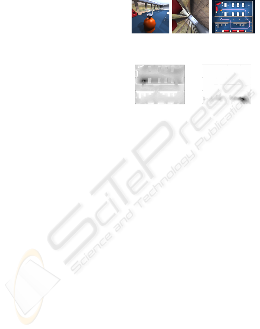
Figure 5: Plots of the dissimilarity between view descrip-

tors obtained at different positions of the simulated envi-

ronment and all the reference views. The grid consists of

4636 views at a spacing of 0.2 m. Dark areas mark likely

positions; white crosses mark the true position. The right

image additionally uses the rotation invariant preﬁltering.

images can be projected onto a hemisphere. To ex-

tend this to a full spherical signal we employ suitable

reﬂection at the equator before approximating the sig-

nal by a SH expansion. Of course this representation

can be obtained directly from the 2D images.

Prior to performing any localization of the robot,

we must create a set of reference frames and calcu-

late its corresponding view descriptors. For our lo-

calization experiment, we have also rendered a series

of frames with the simulated robot moving along a

path (Fig. 4). Note that these positions are in general

not aligned with the grid, neither is the orientation of

the robot aligned with the direction of the reference

frames.

The images in Fig. 5 are maps of the simulated en-

vironment showing a measure corresponding to the

likelihood of the robot location, calculated at discrete

positions along the motion path.

6.2 Hemispherical Camera System

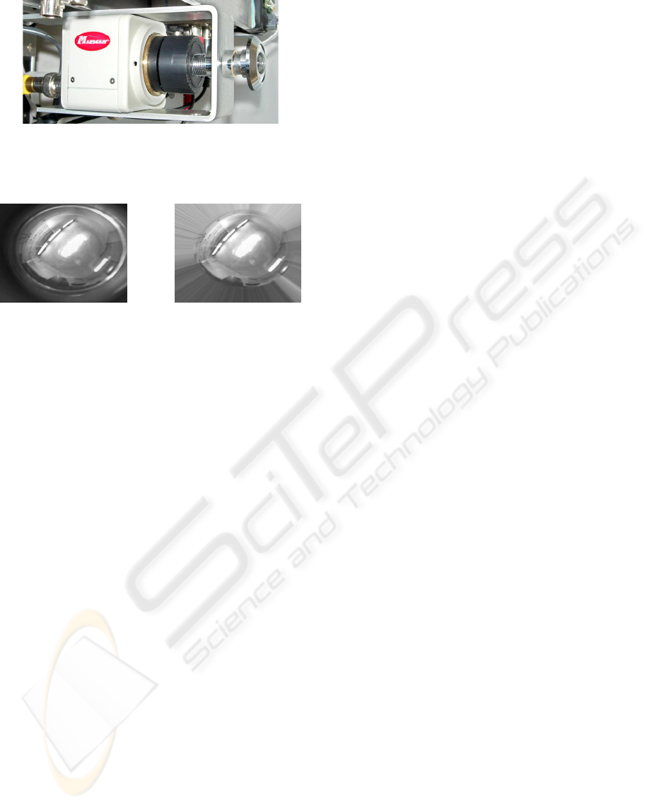
Hardware. To acquire hemispherical wide-angle im-

ages using a real camera, we have designed a low-cost

camera system with a ﬁsheye lens based on the ideas

presented in (Dietz, 2006).

As shown in Fig. 6, the camera system consists

of a cheap door peephole attached to a low-cost b/w

CCTV camera with a 12 mm lens, which is used to

perform ocular projection.

The optical quality of such a system is of course

VIEW-BASED ROBOT LOCALIZATION USING ILLUMINATION-INVARIANT SPHERICAL HARMONICS

DESCRIPTORS

547

(a)

(b)

(c)

(d)

Figure 6: Low-cost camera system based on a door peep-

hole lens (a) adapted to a CCTV camera (c). A mounting

frame (d) is used to lock the peephole in a calibrated dis-

tance to the camera lens (b).

Figure 7: Image data prior to (left) and after preprocessing

(right). Note the interpolated area.

not comparable to commercial high-quality ﬁsheye

lenses; however, if proper image preprocessing

and careful calibration is performed, the results are

already quite useful, especially in the light of this

low-cost solution. For our application, these are more

than acceptable, as we do not make use of the spatial

high-frequency components of the images.

Calibration and Preprocessing. The raw images

obtained by our hemispherical camera system are of

course distorted and like any real camera image re-

quire calibration. However, due to the nature of the

extreme wide-angle lens, there is a blind area beyond

the usable FOV in the images, which is preceded by

an unusable region due to reﬂections of the peephole

housing.

For preprocessing, we ﬁrst perform photometric

calibration (multiplicative). To compensate for the ef-

fects of decaying brightness in the outer regions of

the image,we recorded a set of reference images of

a white homogenous area, which were averaged and

normalized to the lower boundary of a suitable upper

brightness percentile. We use the pixel-wise inverse

of the relative brightness as a template, which is then

multiplied with future captured images. To discard

the garbage induced by reﬂexes at the rim of the im-

ages, we only use a safe area of image data. This

leads to an elliptical image area corresponding to a

FOV of approx. 160

◦

. As the usable image data is

not completely hemispherical, we need to use an ap-

propriate interpolation to extend the signal to the full

180

◦

. We use a radial nearest-neighbor interpolation

from the border of our aforementioned safe area for

that purpose (Fig. 7). This makes sure that no addi-

tional discontinuities occur at the equator of a conse-

quent spherical projection. To project the input image

onto the sphere, we need to calibrate our camera sys-

tem. We use the INRIA toolbox (Mei, 2006).

6.3 Real Environment

Illumination Invariance. For our experiments, we

recorded a grid of 374 reference views in an ofﬁce

while the illumination was kept constant. Thereafter,

we recorded several sequences while the robot was

driven through that environment. This was performed

for two cases – one with the same constant illumina-

tion as for the reference grid, whereas in the other case

there were substantial changes, such as switching the

ceiling lighting on and off (Fig. 8).

Since the CCTV camera we used employs a sub-

optimal gain control which cannot be turned off, we

had to use the normalization according to the pre-

sented multiplicative illumation invariant similarity

measure for performing the localization task even un-

der constant illumination. This method fails, however,

for the second sequence with more severe changes in

illumination, clearly indicating the need for a statisti-

cal model.

To model the typical illumination changes in

that room, we recorded a global training set at a

designated location, which was used as input to a

PCA model. Dissimilarity maps using the resulting

PCA based distance measure show distinctly better

results even where the multiplicative illumation

invariant similarity measure could not cope with the

input (Fig. 8). The results are very promising in the

light that the given illumination changes covered

even extreme cases.

Interpolation. To evaluate whether the detour of

recording all the reference views of a densely spaced

grid is actually necessary to obtain sufﬁciently dis-

tinctive localization results, we computed another ref-

erence grid where the view descriptors in every sec-

ond row and column were obtained through bilinear

interpolation.

In Fig. 9, we show that there are only little differ-

ences between results using a full resolution reference

grid with a spacing of 0.2 m and one obtained by in-

terpolation of a half resolution grid. This applies es-

pecially to the location of the dissimilarity minima.

This encourages the usage of interpolated grids to ob-

tain smoother localization results with more reliable

minima detection.

VISAPP 2008 - International Conference on Computer Vision Theory and Applications

548

(a) Reference image. (b) Illumination changes

and rotation.

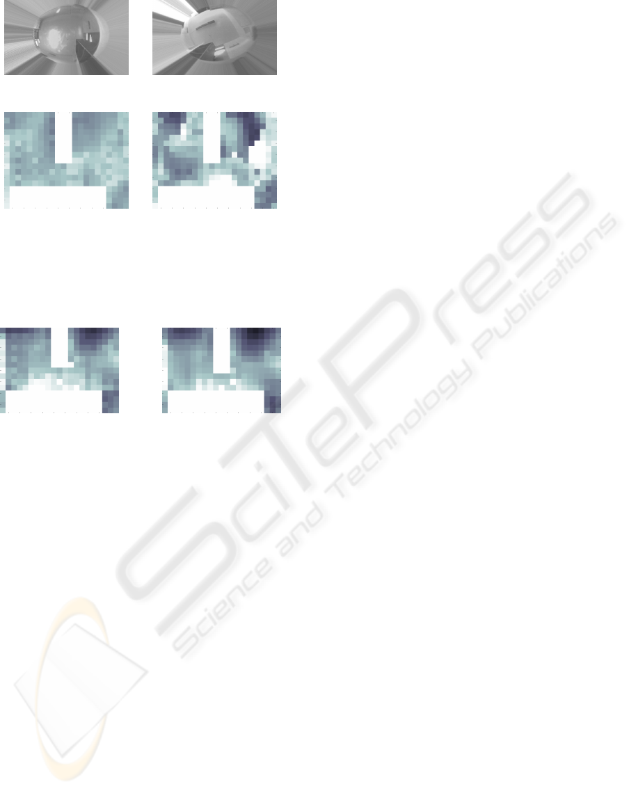
Figure 8: Illumination changes. Dissimilarity maps show-

ing the behavior of different distance measures when ap-

plied to views with substantial illumination changes vs. the

illumination used to record the reference grid. The true po-

sition is at the upper right.

(a) full resolution grid at

0.2 m pixel spacing

(b) interpolated from

half resolution grid

Figure 9: Interpolation. Dissimilarity maps using real data

with the same constant illumination as for recording the ref-

erence grid. Note that both results show only minor differ-

ences.

7 OUTLOOK

So far, only a small fraction of methods to achieve

illumination invariant robot localization have been in-

vestigated in our work. Learning typical effects of

illumination changes for the PCA model at each loca-

tion induces a high effort during the learning phase.

Therefore, other methods should be considered as

well: The generalization from a SH representation

of image signals to a SH representation of feature

images could be useful, e. g. using gradient images

(Reisert and Burkhardt, 2006). Furthermore we could

investigate the beneﬁts of using color images and pho-

tometric invariants (Mileva et al., 2007).

Concerning the interpolation of view descriptors,

a better understanding of the effects which transla-

tions have on the view descriptors will be crucial.

This will be particularly important to further reduce

the required density of the reference view grid. In

connection to this, a differential analysis will provide

a measure to estimate a viable maximum distance be-

tween reference views that still can be interpolated

without excessive error. On the other hand, more so-

phisticated interpolation methods might improve the

localization results.

To speed up and robustify the process of robot lo-

calization, we propose to use more advanced preﬁlter-

ing of unlikely positions. Further invariants can be

determined from applying point-wise non-linear func-

tions on the original or the spherical image signal be-

fore expanding in SH (Schulz et al., 2006). The use

of phase information in addition to the energy spectra

used so far could make the rotation invariant match-

ing of view descriptors more discriminant, resulting

in less views which misleadingly pass the ﬁltering.

An issue that still needs further investigation is

the handling of occlusions, and we proceed towards

this goal. A statistical model for spherical signals

which allows for a correct interpolation of missing

data serves as a highly practical means for compar-

ing/matching/correlating incomplete omnidirectional

data (M

uhlich and Mester, 2004). It allows to com-

pare a given signal with other signals stored in a

database even if the input signal contains areas where

the signal value is not known or very largely de-

stroyed. The potential and usefulness of a statistically

correct procedure for comparing incomplete data can-

not be overestimated.

REFERENCES

Blaer, P. and Allen, P. (2002). Topological mobile robot lo-

calization using fast vision techniques. In Proc. ICRA,

volume 1, pages 1031–1036.

Burel, G. and Henoco, H. (1995). Determination of the

orientation of 3D objects using Spherical Harmonics.

Graphical Models and Image Procesing, 57(5):400–

408.

Dietz, H. G. (2006). Fisheye digital imaging for under

twenty dollars. Technical report, Univ. of Kentucky.

http://aggregate.org/DIT/peepfish/.

Friedrich, H., Dederscheck, D., Krajsek, K., and Mester, R.

(2007). View-based robot localization using Spher-

ical Harmonics: Concept and ﬁrst experimental re-

sults. In Hamprecht, F., Schn

orr, C., and J

ahne, B.,

editors, DAGM 07, number 4713 in LNCS, pages 21–

31. Springer.

Gonzalez-Barbosa, J.-J. and Lacroix, S. (2002). Rover

localization in natural environments by indexing

panoramic images. In Proc. ICRA, pages 1365–1370.

IEEE Computer Society.

Groemer, H. (1996). Geometric Applications of Fourier Se-

ries and Spherical Harmonics. Encyclopedia of Math-

ematics and Its Applications. Cambridge University

Press.

VIEW-BASED ROBOT LOCALIZATION USING ILLUMINATION-INVARIANT SPHERICAL HARMONICS

DESCRIPTORS

549

Jogan, M. and Leonardis, A. (2003). Robust localization

using an omnidirectional appearance-based subspace

model of environment. Robotics and Autonomous Sys-

tems, 45:57–72.

Kazhdan, M., Funkhouser, T., and Rusinkiewicz, S. (2003).

Rotation invariant Spherical Harmonic representation

of 3D shape descriptors. In Kobbelt, L., Schr

oder, P.,

and Hoppe, H., editors, Eurographics Symp. on Ge-

ometry Proc.

Kovacs, J. A. and Wriggers, W. (2002). Fast rota-

tional matching. Acta Crystallographica Section D,

58(8):1282–1286.

ose, B., Vlassis, N., Bunschoten, R., and Motomura,

Y. (2001). A probabilistic model for appearance-

based robot localization. Image and Vision Comput-

ing, 19(6):381–391.

Labbani-Igbida, O., Charron, C., and Mouaddib, E. M.

(2006). Extraction of Haar integral features on om-

nidirectional images: Application to local and global

localization. In DAGM 06, pages 334–343.

Levin, A. and Szeliski, R. (2004). Visual odometry and map

correlation. In CVPR, volume I, pages 611–618.

Makadia, A. (2006). Correspondenceless visual naviga-

tion under constrained motion. In Daniilidis, K. and

Klette, R., editors, Imaging beyond the Pinhole Cam-

era, pages 253–268.

Makadia, A. and Daniilidis, K. (2003). Direct 3D-rotation

estimation from spherical images via a generalized

shift theorem. In CVPR, volume 2, pages 217–224.

Makadia, A. and Daniilidis, K. (2006). Rotation recov-

ery from spherical images without correspondences.

PAMI, 28(7):1170–1175.

Makadia, A., Sorgi, L., and Daniilidis, K. (2004). Rotation

estimation from spherical images. In ICPR, volume 3.

Mei, C. (2006). Omnidirectional calibration toolbox. http:

//www.robots.ox.ac.uk/

cmei/Toolbox.html.

Menegatti, E., Maeda, T., and Ishiguro, H. (2004). Image-

based memory for robot navigation using properties

of the omnidirectional images. Robotics and Au-

tonomous Systems, 47(4).

Menegatti, E., Zoccarato, M., Pagello, E., and Ishiguro, H.

(2003). Hierarchical image-based localisation for mo-

bile robots with Monte-Carlo localisation. In Proc.

European Conference on Mobile Robots, pages 13–

20.

Mester, R., Aach, T., and D

umbgen, L. (2001).

Illumination-invariant change detection using a sta-

tistical colinearity criterion. In Pattern Recognition,

number 2191 in LNCS.

Mileva, Y., Bruhn, A., and Weickert, J. (2007).

Illumination-robust variational optical ﬂow with pho-

tometric invariants. In Hamprecht, F., Schn

orr, C., and

ahne, B., editors, Pattern Recognition, volume 4713

of LNCS, pages 152–162. Springer.

uhlich, M. and Mester, R. (2004). A statistical uniﬁcation

of image interpolation, error concealment, and source-

adapted ﬁlter design. In Proc. SSIAI, pages 128–132.

IEEE Computer Society.

Pajdla, T. and Hlavac, V. (1999). Zero phase representa-

tion of panoramic images for image based localiza-

tion. In Computer Analysis of Images and Patterns,

pages 550–557.

Reisert, M. and Burkhardt, H. (2006). Invariant features for

3D-data based on group integration using directional

information and Spherical Harmonic expansion. In

Proc. ICPR 2006, LNCS.

Schulz, J., Schmidt, T., Ronneberger, O., Burkhardt, H.,

Pasternak, T., Dovzhenko, A., and Palme, K. (2006).

Fast scalar and vectorial grayscale based invariant fea-

tures for 3D cell nuclei localization and classiﬁcation.

In Franke, K. and al., E., editors, DAGM 2006, num-

ber 4174 in LNCS, pages 182–191. Springer.

Steinbauer, G. and Bischof, H. (2005). Illumination

insensitive robot self-localization using panoramic

eigenspaces. In RoboCup 2004.

The Blender Foundation (2007). Blender. http://www.

blender.org.

Thrun, S., Burgard, W., and Fox, D. (2005). Probabilistic

Robotics. The MIT Press.

Turk, M. and Pentland, A. (1991). Eigenfaces for recogni-

tion. J. of Cognitive Neuroscience, 3(1).

Weisstein, E. W. (2007). Legendre polynomial. A Wol-

fram Web Resource. http://mathworld.wolfram.

com/LegendrePolynomial.html.

VISAPP 2008 - International Conference on Computer Vision Theory and Applications

550