AUTOMATIC SHOT BOUNDARY DETECTION USING

GAUSSIAN MIXTURE MODEL

A. Adhipathi Reddy and Sridhar Varadharajan

Applied Research Group, Satyam Computer Services Ltd.

Keywords: Shot boundary detection, Gaussian mixture model, video analysis.

Abstract: The basic step for video analysis is the detection of shots in a given video. A shot is sequence of frames

captured in a single continuous action in time and space using a single camera. The boundary between two

adjacent shots may be an abrupt change (hard cut) or gradual change. In literature, many shot boundary

detection algorithms have been proposed for detecting the hard cut or gradual changes like fadein/out and

dissolve. The performance of these algorithms degrades with zooming, lighting change conditions, and fast

moving type of videos. In this paper, a novel algorithm based on Gaussian Mixture Model (GMM) is

developed for shot boundary detection. The behavior of GMM with abrupt and gradual change is used for

detection of hard cut, fadein/out and dissolve. Experimental results shows credibility of the proposed

algorithm with zooming, lighting change conditions, and fast moving type of videos.

1 INTRODUCTION

With the overwhelmed collection of videos over

Internet and other video libraries, automatic video

analysis for semantic indexing and retrieval has

emerged as a promising area of research. The

foremost step in any video analysis is the detection

of shots in a video. Some of the common methods

used for detecting the shot boundary (SBD) are pixel

difference, histogram comparison, edge change,

compression ratio, and motion vectors. Performance

comparison of these algorithms can be found in

(Lienhart, 1999).

Zhang et al. (Zhang, 1995) proposed a method

in which block by block difference is used instead of

pixel difference to overcome sensitivity to camera

motion and noise. To improve the performance of

histogram based SBD, Huang et al. (Huang, 2003)

have proposed the use of row and column

histograms in addition to global histogram.

Hardware implementation of the local histogram

based SBD can be found in (Boussaid, 2007).

However, histogram based methods lack spatial

information and are also sensitive to changes in

illumination and noise.

To avoid costly decompression of frames, many

compression domain techniques based on

compression difference or motion vectors (Tardini,

2005) have been proposed. Zabih et al. (Zabih,

1995) have proposed SBD based on determining the

number of incoming and outgoing edge pixels called

edge change ratio (ECR). Hard and gradual changes

are detected by analyzing the characteristics of ECR

time series. To make the SBD algorithm robust,

many researchers have proposed to use multiple

features (Bruyne, 2006) (Fang, 2006). Even though

the performance of these algorithms are better than

histogram and pixel difference based methods, the

complexity in extracting the feature vectors is high

making them less suitable for real time applications.

To overcome the above drawbacks, in this

paper a GMM based shot boundary detection

algorithm is proposed. At each frame, probability

that the present frame fits into the GMM estimated

up to the previous frame is calculated. The

probabilities obtained at each frame are analyzed to

detect hard cut and gradual change. As the GMM are

inherently immune to noise and can handle the

lighting change condition efficiently, the proposed

algorithm can detect the shot boundaries more

efficiently. The remainder of the paper is organized

as follows. Section 2 describes the GMM and the

proposed algorithm. Experimental results are

presented in section 3 and the concluding remarks

are given in section 4.

547

Adhipathi Reddy A. and Varadharajan S. (2008).

AUTOMATIC SHOT BOUNDARY DETECTION USING GAUSSIAN MIXTURE MODEL.

In Proceedings of the Third International Conference on Computer Vision Theory and Applications, pages 547-550

DOI: 10.5220/0001084705470550

 SciTePress

2 SHOT BOUNDARY

DETECTION ALGORITHM

In surveillance applications, GMMs are widely in

use for modeling the static background for detecting

the foreground objects (Stauffer, 1999). Mo and

Wilson (Mo, 2004) used multiresolution GMMs to

capture both spatial and statistical aspects of the

video. Based on the log-likelihood derived from the

model, significant scene changes are detected. Next,

we give an introduction to GMM, following which

the proposed algorithm is discussed.

2.1 Gaussian Mixture Model

Gaussian mixture models are the probabilistic

models for representing a distribution. GMM can

also be viewed as a form of generalized radial basis

function network in which each Gaussian

component is a basis function or `hidden' unit. Let us

represent the

k Gaussian component in a mixture

model by

()

∑

, where

is the mean value

and

∑ is the variance. The probability that a sample

value

belongs to a GMM is given by

()()

∑

∑Ν∗=

kkk

xpwxp

,/)(

(1)

where

n is the number of components in a Gaussian

mixture and

w is the normalized weight factor

associated with that Gaussian. Gaussian probability

density function for

()

∑

is calculated by

()()

)()(

exp

μμ

−∑−−

−

∑

=∑Ν

(2)

An expectation-maximization algorithm is used

for fitting the GMM with a given set of training data.

This algorithm is the best approach to train the

stationary data. As the present algorithm is dealing

with time varying data, this maximum likelihood

algorithm is not suitable. Hence, an approximation

to the expectation-maximization is used for updating

the GMM over the time.

2.2 Proposed Method

The algorithm is implemented in compression

domain. Partial decoding of the data is required for

DC value extraction. This is another added

advantage of the proposed algorithm. Each

component is modeled with separate Gaussian

mixture.

GMMs are initialized for each block with first

frame of the sequence. First component of each

GMM is initialized with the DC values

corresponding to R, G, and B as given below

BGR ===

111

μμμ

(3)

where

R 11

μμ

and

are the mean values of

the first Gaussian.

GR ,

, and

are the R, G,

and B DC components of

i block. Rest of the

Gaussian components are initialized with zero value.

Weights and variances of all the components are

initialized with initial parameters.

To update the model from frame to frame, for

every block of current frame find the best matching

GMM in

neighborhood blocks of the previous

frame. The probability of fitting

block’s DC

value in the previous frame’s

block GMM is

calculated by distance function

(

)

∑

−

BGR

jid

),(

(4)

Equation 4 is approximately equal to the

Mahalanobis distance with off diagonal elements of

covariance matrix zero. Zero off diagonal elements

means, R, G, and B components are independent and

have the same variance.Even though this assumption

is not true, it avoids us to do costly matrix inversion

at the expense of some accuracy. Using equation 4,

find the minimum distance Gaussian component and

corresponding block number as given below

where

is the

neighborhood of

i block in

previous frame.

For finding the shot boundary and shot

transition type, count the number of blocks with

TD >

, where

is the distance threshold. Let us

represent this count with

. If

is plotted against

the frame number, it exhibits a different

characteristic for hard cuts, dissolves, and fades as

shown in Figure 1. From Figure 1(a), it can be

observed that, for hard cut the change in the value of

is sudden. After a sudden change there is a

gradual decrease of

value in the following

frames as GMM gets updated.

(

)

()

),(minarg

jidl

jidD

(5)

VISAPP 2008 - International Conference on Computer Vision Theory and Applications

548

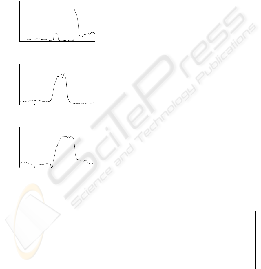
Dissolves type of shot boundary transition

exhibits a bell shape as shown in Figure 1(b). During

the dissolve, the number of blocks with no best fit

GMM increases gradually. After a few frames, as

the GMMs get updated over a few blocks, the

Mahalanobis distance curve decreases gradually. In

case of fade-ins/fade-outs, as DC values

increase/decrease continuously, the blocks without

best fit GMMs peak for a few frames. This looks

like a trapezoidal shape as given in Figure 1(c).

Flickering type of lighting conditions can be

detected by finding

NNN ,,,

for other Gaussian

components similar to that of finding

. If there is a

sudden change in

and at the same time if for any

other Gaussian component

k ,

is less, it is

characterized as flickering.

The updating of GMM of blocks of current

fame is as given in equation 6

()

αα

μαα

+−=

−+∑−=∑

+−=

−

)1(

ttt

(6)

where I is R, G, or B component and

is the

learning rate. If no matching GMM is found, then

assign the spatial corresponding block GMMs of

previous frame and initialize the last component of

GMM with the DC component of the current block.

After updating the GMM, weights are normalized.

Based on the normalized weights, components of

GMM are rearranged.

3 EXPERIMENTAL RESULTS

In this section, performance of the proposed

algorithm is tested with different type of videos. For

initialization of a GMM, initial weight and variance

are taken as 0.2 and 225 respectively. The number of

Gaussian components is selected as 3. Threshold

value

0.1

and

2.0

is chosen after testing

with different types of videos.

Experimental results with the proposed method are

presented for four different test sequences, namely,

news, documentary, soccer, and basketball. These

sequences are selected as they have lot of zooming,

light changing, and fast moving effects. For all test

sequences, the ground truths are generated manually

with precise location and type of transition. Ground

truth of these sequences is given in Table 1.

Performance of the algorithm is measured by using

three types of measurements:

• Correct detection ratio is the ratio of shot

transitions correctly detected to the actual

number of transitions.

• Miss detection ratio is the ratio of number of

shot transitions not detected to the actual

number of shot transitions.

• False detection ratio is the ratio of number

of shot transitions falsely detected to the

actual number of shot transitions

Table 1: Ground truth of test sequences for hard cut (H),

dissolve (D) and fades (F).

Test sequence Duration

(min)

H D F

ews 7.00 44 0 0

Documentary 12.00 87 16 2

Soccer 11.00 45 30 0

Basketball 15.36 95 41 0

0.2

0.4

0.6

0.8

0 20406080100

frame number

mahalanobis distance

(a) Hard cut

0.2

0.4

0.6

0.8

0 20406080100

Frame number

Mahalanobis distanc e

(b) Dissolves

0.2

0.4

0.6

0.8

0 20406080100

frame number

Mahalanobis dis tance

Figure 1: Typical pattern of Mahalanobis distance vs

frames for hard cut

dissolve and fades.

AUTOMATIC SHOT BOUNDARY DETECTION USING GAUSSIAN MIXTURE MODEL

549

Table 2: Performance results for hard cut (H), dissolve (D)

and fades (F) detection.

The results with the proposed method are presented

in Table 2. From Tables 1 and 2 it can be observed

that hard cut detection ratio is 99.67% while dissolve

detection ratio is 79.3%. Only two fade-outs are

present in the documentary sequence and the two are

detected correctly. Miss detection ratio for hard cut

is 3.32% and for dissolve it is 20.22%. False

detection ratio for hard cut and dissolve are 21% and

9.2% respectively. Results indicate that the

performance of hard cut detection is very high and in

most cases, dissolve detection is also correct. Our

observation is that false detections occur in closeup

shots. Specifically, these can be observed very

prominently in the basketball sequence where

players are showed closely while moving fast.

For the qualitative evaluation of the proposed

method, we refer the results presented with various

algorithms in (Lienhart, 1999). In (Lienhart, 1999),

Lienhart evaluated the best known algorithms and

presented improvements to them. With these

improvements, Lienhart achieved correct and false

detection ratios for hard cut as 95% and 5% and for

dissolve as 80% and 20% respectively. Even though,

out test data is not as big as that Lienhart used, the

results do bring out the merits of our method. As we

have selected by carefully considering the various

types of camera actions and events, the results can

be considered as consistent over a large data set as

well.

4 CONCLUSIONS

This paper presents a novel algorithm for shot

boundary detection using Gaussian mixture models.

Performance of the algorithm is verified by testing

with different types of test sequences. Results

indicate that proposed method can handle zooming,

lighting change, and fast moving scenes effectively.

However, the performance degrades with closeup

shots with fast moving camera action or activity.

These are due to the delay in updating the GMMs.

Handling of these types of problems for reducing the

false detection is considered in part of our on going

work.

REFERENCES

Lienhart, R., 1999. Comparison of automatic shot

boundary detection algorithms. In proc. IS &T/SPIE

Storage and Retrieval for Image and Video Databases

VII. vol. 3656, pp 290-321.

Zhang, H., Kankanhalli, A., Smoliar, S.W., 1995.

Automatic partitioning of full-motion video.

Multimedia Systems. vol. 1, pp. 533-544.

Huang, X., Wei, G., Petrushin, V.A., 2003. Shot boundary

detection and high-level feature extraction for the

TREC video evaluation 2003. NIST TRECVID 2003.

Boussaid, L., Mtibaa, A., Abid, M., Paindavoine, M.,

2007. A real time shot cut detector: Hardware

implementation. Computer Standards & Interfaces.

Vol. 29, Issue 3, Pages 335-342.

Tardini, G., Grana, C., Marchi, R., Cucchiara, R., 2005.

Shot detection and motion analysis for automatic

MPEG-7 annotation for sports video. In Int. Conf. on

Image Analysis and Processing, pp. 653-660.

Zabih, R., Miller, J., Mai, K., 1995. Feature-based

algorithms for detecting and classifying scene breaks.

In Proc. ACM on Multimedia. pp. 189–200,

Bruyne, S.D., Wolf, K.D., Neve, W.D., Verhoeve, P.,

Walle, R.V.D., 2006. Shot boundary detection using

macroblock prediction type information. In Workshop

on Image Analysis for Multimedia Interactive

Services. pp. 205-208.

Fang, H., Jiang, J., Feng, Y., 2006. A fuzzy logic approach

for detection of video shot boundaries. Pattern

Recognition. Vol. 39, , Pages 2092-2100.

Stauffer, C., Grimson, W.E.L, 1999. Adaptive background

mixture models for real-time tracking. In Proc. of Int.

Conf. on Computer Vision and Pattern Recognition.

Vol. 2, pp.246-252.

Mo,X.,Wilson,R.,2004. Video modeling and segmentation

using Gaussian mixture models. In Proc. of Int. Conf.

on Pattern Recognition, Vol. 3, pp 854-857.

Test sequence

Correct

Detection

False Detection

H D F H D F

News 44 0 0 0 0 0

Documentary 87 8 2 10 2 2

Soccer 41 24 0 8 2 0

Basket-ball 90 37 0 39 4 7

VISAPP 2008 - International Conference on Computer Vision Theory and Applications

550