
ESTIMATING CAMERA ROTATION PARAMETERS FROM A
BLURRED IMAGE
Giacomo Boracchi
a,b
, Vincenzo Caglioti
a
and Alberto Danese
a
a
Dipartimento di Elettronica e Informazione
Politecnico di Milano, Via Ponzio, 34/5 20133 Milano, Italy
b
Tampere International Center for Signal Processing,
∗
Tampere University of Technology, P.O. Box 553, 33101 Tampere, Finland
Keywords:
Blurred Image Analysis, Camera Rotation, Camera Ego-motion, Blur Estimation, Space Variant Blur.
Abstract:
A fast rotation of the camera during the image acquisition results in a blurred image, which typically shows
curved smears. We propose a novel algorithm for estimating both the camera rotation axis and the camera
angular speed from a single blurred image. The algorithm is based on local analysis of the blur smears.
Contrary to the existing methods, we treat the more general case where the rotation axis can be not orthogonal
to the image plane, taking into account the perspective effects that in such case affect the smears.
The algorithm is validated in experiments with synthetic and real blurred images, providing accurate estimates.
1 INTRODUCTION
This paper concerns images corrupted by blur due to
a camera rotation or to a rotating object in the scene.
When the camera or the captured object are purely ro-
tating, the image blur is determined by only two fac-
tors: the camera rotation axis a and its angular speed
ω. We present a novel algorithm for estimating both
a and ω, by analyzing the blur in a single image.
When the camera rotation axis and the angular
speed are known, the rotationally blurred image can
be restored by image coordinates transformation and
blur inversion. In broad terms, the image is trans-
formed from Cartesian to polar coordinates so that the
blur becomes space invariant and can be inverted us-
ing a deconvolution based algorithm. Estimating cor-
rectly the camera rotation axis and its angular speed
is therefore crucial for restoring these images as small
errors in the polar transformation are amplified by
blur inversion.
On the other hand, estimating a and ω from a sin-
gle image can be also of interest for robotic applica-
tion as these describe the camera ego-motion.
Figure 1 shows an image acquired during camera
rotation. The shapes of the blur smears show that the
∗
This work was partially supported by CIMO, the
Finnish Centre for International Mobility (fellowship num-
ber TM-07-4952)
Figure 1: A rotationally blurred image.
blur is space variant. Typically, these are assumed
arcs of circumferences, all having the same center.
However, this approach neglects the perspective ef-
fects that occur when the rotation axis is not orthog-
onal to the image plane. The proposed algorithm es-
timates the camera rotation axis in the most general
case when it is not necessarily orthogonal to the im-
age plane. To the best of our knowledge this issue has
never been correctly addressed before.
Besides the early works concerning rotational blur
modeling and restoration, Hong and Zhang (Hong and
Zhang, 2003) addressed the issue of both rotational
blur estimation and removal. Their method is based
on an image segmentation along circumferences to
389
Boracchi G., Caglioti V. and Danese A. (2008).
ESTIMATING CAMERA ROTATION PARAMETERS FROM A BLURRED IMAGE.
In Proceedings of the Third International Conference on Computer Vision Theory and Applications, pages 389-395
DOI: 10.5220/0001085403890395
Copyright
c
SciTePress

V
V
a
b
S
π
π
π
π
c
C ≡P
C
P
a
a
Figure 2: (a) Blurred image formation, a ⊥ π. Blurring
paths are circumferences. (b) Blurred image formation, a
is not orthogonal to image plane π and V ∈ a. Blurring
paths are conic sections on the image plane, while they are
circular when projected on an ideal spherical sensor and on
a plane perpendicular to the rotation axis.
estimate the blur and restore the image separately in
these subsets. Recently, an algorithm for estimating
the camera rotation from a single blurred image has
been proposed (Klein and Drummond, 2005). The al-
gorithm is meant as a visual gyroscope and it is tar-
geted to an efficient implementation. In particular,
this algorithm requires edges in the scene.
All the existing methods, concerning both image
restoration and blur estimation, assume that the blur
smears are arcs of circumferences having the same
center. Therefore these methods are accurate only on
images where the rotation axis is orthogonal to the
image plane.
We present an algorithm for estimating the camera
rotation axis and angular speed in the most general
case, where the rotation axis is not orthogonal to the
image plane. The proposed algorithm is mostly tar-
geted to accuracy rather than efficiency and does not
require the presence of edges in the scene.
2 PROBLEM FORMULATION
We propose an algorithm for estimating the camera
rotation axis a and its angular speed ω by analyzing a
single blurred image acquired during camera rotation.
We assume that the camera is calibrated, the rotation
axis a passes through its viewpoint V, i.e. V ∈ a, and
w is constant. Figure 2.a illustrates the situation typi-
cally considered in literature, where the rotation axis
is perpendicular to image plane π. The principal point
P and the intersection between the image plane and
the rotation axis C = π∩a then coincide. Analogous
blur is obtained when a ⊥π and V /∈a, but the capture
scene is planar and parallel to π (Ribaric et al., 2000).
In this work we consider the most general situa-
tion, illustrated in Figure 2.b, where a is not orthogo-
nal to π and the camera viewpoint V ∈ a.
2.1 Image Blur
A blurring path is defined as the set of image pixels
that a viewing ray intersects during a camera rotation
of 2π around axis a. Figure 2 illustrates examples
of blurring paths. In rotationally blurred images ev-
ery pixel is merged with neighboring pixels from the
same blurring path, see Figure 1. The blur is there-
fore space variant and can not be represented as a lin-
ear shift invariant system. We therefore model the ro-
tational blur by an operator K on the original image
y (Bertero and Boccacci, 1998) so that the observed
(blurred and noisy) image z is
z(x) = K
y
(x) + η(x) x = (x
1
,x
2
) ∈ X , (1)
x being the coordinates in the discrete image domain
X and η ∼ N(0,σ
2
η
) is white Gaussian noise. The blur
operator K can be written as
K
y
(x) =
Z
X
k(x,s)y(s)ds. (2)
where k(x, •) is a kernel
k(x,•) = A
θ,e
(•), (3)
and A
θ,e
corresponds to the point spread function
(PSF) at x. A
θ,e
being an arc the blurring path at x, i.e.
is an arc of conic section having tangent line with di-
rection θ and arc length e. The parameters θ,e varies
between image pixels according to the rotation axis a.
Other blurring effects, such as the out of focus blur,
lenses aberrations and camera shake, are not consid-
ered.
3 THE ALGORITHM
The proposed algorithm is based on three steps: in the
first step the lines tangent to blurring paths at some
image pixels are estimated (Section 3.1). In the sec-
ond step, these lines are used in a voting procedure for
estimating the rotation axis a (Sections 3.2 and 3.3).
The third step consists of the angular speed ω estima-
tion (Section 3.4).
3.1 Blur Tangent Direction Estimation
Image blur is analyzed within N image regions taken
around selected pixels {x
i
}
i=1,..,N
. There are no
particular requirements in selecting {x
i
}
i=1,..,N
, but
avoiding smooth areas while covering uniformly the
image. Therefore we take the local maxima of Harris
corner measure (Harris and Stephens, 1988), or when-
ever these do not cover uniformly the image, we take
{x
i
}
i=1,..,N
on a regular grid.
VISAPP 2008 - International Conference on Computer Vision Theory and Applications
390
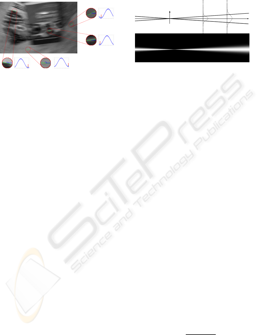
Figure 3: Rotationally blurred image and plots of direc-
tional derivatives energy in four regions.
Blur is analyzed using the approach proposed by
Yitzhaky et al (Yitzhaky and Kopeika, 1996) for esti-
mating the direction of blur “smears” by means of di-
rectional derivative filters. This method, proposed for
space invariant blurs with PSF having vectorial sup-
port, assumes the image isotropic. The blur direction
b
θ is estimated as the direction of the derivative filter
d
θ
having minimum energy response
b
θ = arg min
θ∈[0,π]
||(d
θ
⊛ z)||
1
, (4)
where ⊛ denotes the convolution and
||(d
θ
⊛ z)||
1
=
∑
x∈X
|(d
θ
⊛ z)(x)| the ℓ
1
norm.
Equation (4) is motivated by the fact that the blur
removes all the details and attenuates edges of y along
blur direction. Therefore the blur direction can be
determined by the directional derivative filter having
minimum energy. This method can not be directly
applied to rotationally blurred images, as the blur is
not space invariant because in every pixel the circum-
ference approximating the blurring path (i.e the PSF)
changes.
At x
i
, the center of each regionU
i
, we estimate the
direction θ
i
of the line l
i
tangent to the blurring path
in x
i
, as
θ
i
= arg min
θ∈[0,π]
∑
x
j
∈U
i
w
j
(d
θ
⊛ z)(x
j
)
2
. (5)
being w a window function rotationally symmetric
with respect to the center. By using Gaussian dis-
tributed weights, it is possible to reduce the influence
of pixels in Equation (5) with the distance from x
i
. We
adopted the 3 tap derivative filters presented in (Farid
and Simoncelli, 2004) for blur analysis in Equation
(5). These filters have been selected as they provide
good accuracy and as they are separable. Experimen-
tally the ℓ
2
norm gave better results than the ℓ
1
norm.
Figures 3 shows
∑
x
j
∈U
i
w
j
(d
θ
⊛ z)(x
j
)
2
as a
function of θ ∈[0,π] within regions of the blurred im-
age containing isotropic textures or edges. Regions
p
1
p
2
1
k
Figure 4: Weight function used for the votes spread.
containing edges, as pointed out in (Klein and Drum-
mond, 2005), can be exploited for estimating the cam-
era rotation: in z only edges tangent to the blurring
paths are preserved. Formula (5) gives accurate re-
sults also when U
i
contains a blurred edge, as the di-
rection minimizing the derivatives energy is the edge
direction, i.e the blur tangent direction.
3.2 Voting Procedure for Circular
Blurring Paths
When the camera optical axis and the rotation axis a
coincide, the blurring paths are circumferences cen-
tered in C = π ∩a, see Figure 2.a. Circular blurring
paths are obtained also when a is parallel to the op-
tical axis and the scene is planar and parallel to the
image plane (Ribaric et al., 2000; Hong and Zhang,
2003). In this case C can be determined by a Gener-
alized Hough Transform (Ballard, 1987).
The Generalized Hough Transform is a procedure
for computing robust solution to a problem, given
some input data. The procedure is developed by
means of a parameters space P, which is the set of
all the possible solutions. A vote is assigned to ev-
ery parameter that satisfy a datum and then summed
to the votes coming from the other data. After having
considered all the data, the parameter that receivedthe
highest vote is taken as a solution.
In our case P is a discrete grid of all the pos-
sible location for C ∈ π and data are the pairs
(x
i
,θ
i
) i = 1, ..,N. Note that C could be outside of
the image grid X. Every data (x
i
,θ
i
) identifies a line
l
i
, the line tangent to the blurring path at x
i
. The set
of all the possible rotation centers C, given the line l
i
,
is the line perpendicular to l
i
and passing through x
i
.
It is worth to take into account the root mean
square error of each θ
i
i.e.
σ
i
=
q
E[(θ
i
−θ
∗
i
)
2
] (6)
where θ
∗
i
represents the true tangent blur direction
at x
i
and E[•] the mathematical expectation. Since
ESTIMATING CAMERA ROTATION PARAMETERS FROM A BLURRED IMAGE
391

we can not directly compute σ
i
, we approximate it
with an indirect measurement: for example consid-
ering the amplitude of the area near θ
i
in the energy
function minimized in (5) or considering σ
i
propor-
tional to σ
η
(1). Noise standard deviation is estimated
using (Donoho and Johnstone, 1994). Given a datum
(x
i
,θ
i
), we assign a full vote to all the exact solutions
and we spread smaller votes to the neighboring pa-
rameters, according to the errors in θ
i
.
Let now p = (p
1
, p
2
) represent a coordinate sys-
tem in the parameters space and assume θ
i
= 0 and
x
i
= p
i
= (0, 0). Let now model the vote spread
assuming that along the line p
1
= 1 the errors are
distributed as σ
i
√
2π ·N(0,σ
i
). We model the vote
spread so that along line p
1
= k, the votes are still
Gaussian distributed with a full vote at the exact so-
lution (k,0) and for neighboring parameters the votes
depend only on the angular distance from θ
i
, see Fig-
ure 4. Therefore the following weight function is used
for distributing the votes in the parameter space (when
x
i
= p
i
= (0,0) and θ
i
= 0),
v
i
(p
1
, p
2
) = e
−
p
2
2
1+p
2
1
σ
2
i
, (7)
The votes weight function v
i
, associated to other data
(x
i
,θ
i
), correspond to Equation (7) opportunely ro-
tated and translated. When all pairs (x
i
,θ
i
) i = 1, .., N
have been considered, the parameter that received the
highest vote is taken as the solution, i.e.
ˆ
p = argmax
p∈P
V (p), being V (p) =
N
∑
i=1
v
i
(p). (8)
The coordinates of C = π∩a are determined from
ˆ
p.
3.3 Conic Section Blurring Paths
Assuming circular blurring paths reduces the com-
plexity load but gives inaccurate solutions whenever
a is not perpendicular to π. We present an algorithm
for estimating a and ω when V ∈ a and a is in a gen-
eral position w.r.t. π. In particular, if we call π
C
a
plane perpendicular to a, π
C
is obtained by two rota-
tions of α and β from π. We do not consider V /∈a as
in this case the blur would depend on the scene depth.
Votes in the parameters space show at a glance
what happens assuming circular blurring paths when
a is not orthogonal to π. Figure 5.a shows a blurred
image produced when the plane orthogonal to a forms
angles α
∗
= 45
◦
and β
∗
= 0
◦
with π. If we treat the
blurring paths as circumferences, the votes in the pa-
rameters space do not point out a clear solution, as
shown in Figure 5.b and 5.c.
Directions θ
i
obtained from (5) represent the blur-
ring paths tangent direction, even when the blurring
paths are conic sections. But the blurring paths them-
selves are not circumferences, thus lines perpendic-
ular to these tangent lines do not cross at the same
point.
From basic 3D geometry considerations, and as
pointed out in (Klein and Drummond, 2005), it fol-
lows that the blurring paths are circumferences on
an ideal spherical sensor S, Figure 2.b. Then, if we
project the image from π on S surface, the blurring
paths become circumferences. Each of these circum-
ferences belongs to a plane and all these planes have
the same normal: the rotation axis a. Let now con-
sider one of these planes, π
C
, tangent to the sphere.
The projections of the blurring paths on π
C
are cir-
cumferences, Figure 2.b.
The plane π and the plane π
C
are related by a pro-
jective transformation determined by two parameters,
namely (α,β), the angles between the two planes. De-
fine the map M
α,β
: π 7→ π
α,β
as the projection from V
between π and π
α,β
, which is the plane tangent to S,
forming angles (α,β) with π (Rothwell et al., 1992).
We search for (α,β) that project the blurring paths
into circumferences, by modifying the voting proce-
dure of Section 3.2.
There is no need to transform the whole image
with M
α,β
as each l
i
, the line tangent to the blur-
ring path at x
i
, can be directly mapped via M
α,β
.
Let v
α,β
i
be the weight function (7) associated to data
(x
i
,θ
i
) i = 1,..,N mapped via M
α,β
. The parameters
pair identifying the plane π
C
is estimated as
(
ˆ
α,
ˆ
β) = argmax
α,β
V
α,β
(
ˆ
p
α,β
), (9)
being
ˆ
p
α,β
= argmax
p∈P
V
α,β
(p), V
α,β
(p) =
N
∑
i=1
v
α,β
i
(p).
(10)
Figure 5.d and 5.e represent the votes in case the
data have been transformed according to the correctly
estimated parameters
ˆ
α = 45
◦
,
ˆ
β = 0
◦
. These votes
are much more concentrated than votes in Figure 5.b
and 5.c.
Once
ˆ
α and
ˆ
β have been estimated, the cam-
era rotation axis a is determined and it is possible
to map the image z to M
ˆ
α,
ˆ
β
(z). As said before, in
M
ˆ
α
,
ˆ
β
(z) the blurring paths are circumferences cen-
tered at M
ˆ
α,
ˆ
β
(C) ≡ π
C
∩a and it is therefore possible
to transform M
ˆ
α
,
ˆ
β
(z) in polar coordinates for estimat-
ing the angular speed.
3.4 Angular Speed Estimation
Once C has been determined, it is possible to trans-
form M
ˆ
α,
ˆ
β
(z) (the image projected on π
C
) on a polar
VISAPP 2008 - International Conference on Computer Vision Theory and Applications
392

Figure 5: (a) Rotationally blurred image with rotation axis α
∗
= 45
◦
,β
∗
= 0
◦
. (b) Votes assuming circular blurring paths, (c)
votes contours. (d) Votes obtained transforming the data with
ˆ
α = 45
◦
,
ˆ
β = 0
◦
, (e) votes contours. The maximum vote in (d)
is 33% higher than the maximum vote in (b). This is due to the fact that transforming the data with M
45,0
the blurring paths
become circumferences having the same center.
Figure 6: Still and rotationally blurred synthetic images.
First row, left to right: Boat (α
∗
= 20
◦
,β
∗
= 0
◦
), Man-
drill (α
∗
= −20
◦
,β
∗
= 20
◦
) and Lena (α
∗
= 0
◦
,β
∗
= −20
◦
).
Second row: Boat, Mandrill and Lena, rotationally blurred
with an angular speed of 6, 8 and 6 deg/s, respectively, as-
suming 1 second of exposure time. Intersection between
image plane and rotation axis is marked with a red circle.
lattice (ρ,θ) w.r.t to M
ˆ
α,
ˆ
β
(C) (Ribaric et al., 2000).
On the polar lattice, the blur is space invariant with the
PSF directed along lines ρ = const. We estimate the
PSF extent using the method proposed by Yitzhaky
(Yitzhaky and Kopeika, 1996) as this can be applied
to a restricted image area, avoiding lines which con-
tain several pixels of padding introduced by the polar
transformation. The PSF extent, opportunely scaled
by the factor due to the polar lattice resolution, di-
vided by the exposure time gives the camera angular
speed.
4 EXPERIMENTS
The algorithm has been validated both on synthetic
and camera images. Synthetic images of Figure
6 have been generated with a raytracer software
(http://www.povray.org/,) rotating the camera in front
of planar tiles of test images. Blurred images are ob-
Table 1: Boat. Highest votes corresponding to (α,β) in the
parameters space, expressed as a percentage with respect to
the maximum vote.
α β -40 -20 0 20 40
-40 33 52 72 53 48
-20 39 52 83 63 44
0 34 57 83 63 43
20 40 55 100 55 44
40 35 42 62 39 34
Table 2: Refinement around (
ˆ
α,
ˆ
β) from Table 1.
α β -10 0 10
10 71 79 80
20 63 100 74
30 57 82 61
tained averaging all the rendered frames, according to
Equation (1). Ten frames (512x512 pixels, grayscale
0-255) are rendered per each rotation degree. The
blurring paths tangent directions are estimated in 121
equally spaced regions having a 10 pixel radius, using
formula (5).
Table 1 shows V
α,β
(
ˆ
p
α,β
) (the value of the maxi-
mum vote obtained with (α,β)) as a percentage w.r.t
V
ˆ
α,
ˆ
β
(
ˆ
p
ˆ
α,
ˆ
β
) (the maximum vote obtained with (
ˆ
α,
ˆ
β)).
Here (
ˆ
α,
ˆ
β) coincides with (α
∗
,β
∗
), the ground truth.
Table 2 shows the results at a second iteration consid-
ering a refinement around (
ˆ
α,
ˆ
β)).
Table 3 shows results obtained on synthetic im-
ages of Figure 6. Each of them has been tested
adding white gaussian noise with standard devia-
tion 0, 0.5 and 1 and considering α and β in
A = B = {−40
◦
,−20
◦
,0
◦
,20
◦
,40
◦
}. Algorithm per-
formances are evaluated with ∆(α)=|
ˆ
α − α
∗
| and
∆(β)=|
ˆ
β − β
∗
|. ∆(
ˆ
C) and ∆(
ˆ
ω) represent the abso-
lute error between the ground truth and the estimated
values of C = π∩a and ω, respectively.
ESTIMATING CAMERA ROTATION PARAMETERS FROM A BLURRED IMAGE
393
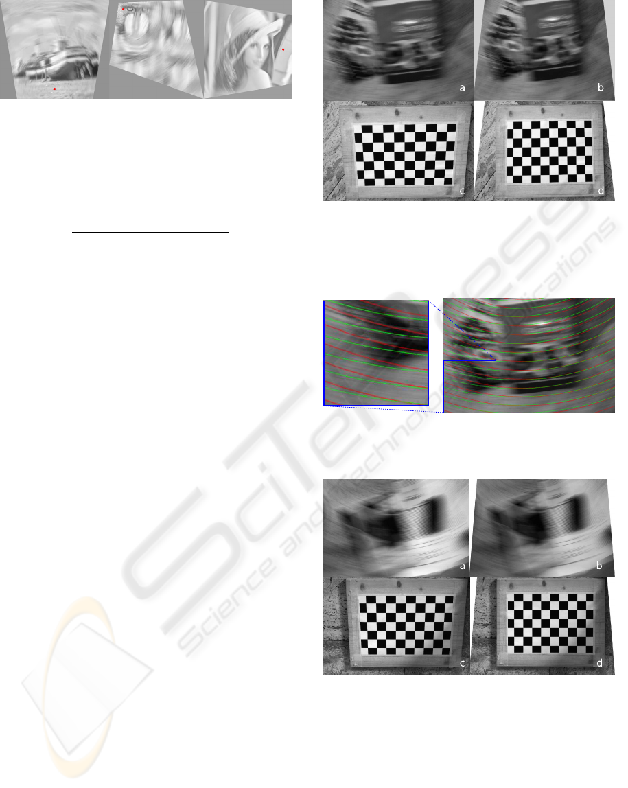
Figure 7: Boat, Mandrill and Lena rectified with the corre-
sponding estimated (
ˆ
α,
ˆ
β). Intersection between the image
plane and the rotation axis is marked with a red circle.
The effectiveness of our algorithm is evaluated as
adv =
V
ˆ
α,
ˆ
β
(
ˆ
p
ˆ
α
,
ˆ
β
) −V
α
2
,β
2
(
ˆ
p
α
2
,β
2
)
V
α
2
,β
2
(
ˆ
p
α
2
,β
2
)
, (11)
being V
α
2
,β
2
(
ˆ
p
α
2
,β
2
) the maximum vote obtained
among other parameters (α,β). The higher this ratio,
the better. Finally, ∆(C
0,0
) and ∆(ω
0,0
) are the corre-
sponding errors obtained assuming circular blurring
paths. Results for noisy images represent the average
over ten different noise realizations.
Results reported in Table 3 show that our algo-
rithm can cope with a reasonable amount of noise,
obtaining regularly better results than the circular blur
assumption. This is more evident in the estimation
of the angular speed, which lacks physical meaning
when the rotation axis is not correctly identified. Fig-
ure 7 shows blurred images of Figure 6 transformed
with the corresponding M
ˆ
α,
ˆ
β
.
Camera images have been captured rotating a
Canon EOS 400D camera on a tripod, assuring that
a is orthogonal to the floor. The ground truth α
∗
and
β
∗
, can be then computed rectifying still images of a
checkerboard on the floor. Figures 8.a and 10.a show
the downsampled RAW converted in grayscale used
to test our algorithm. The blurring path tangent direc-
tions are estimated on 187 uniformly spaced regions,
having 10 pixel radius.
Tables 4 and 5 show the results of the execution
of two iterations of the algorithm on Figure 8.a. The
solution obtained is
ˆ
α = −30
◦
and
ˆ
β = 0
◦
, which
is acceptable as the ground truth, obtained from the
checkerboard, is (−27
◦
,0
◦
). Figure 9 points out the
differences between the blurring paths estimated with
the circular approximation (in red) and the conic sec-
tion paths estimated by our method (in green). As
clearly seen from the detail, the blur is correctly in-
terpeted by the green blurring paths. Figure 10 shows
results on another camera image, having α
∗
= −20
◦
and β
∗
= 0
◦
. After two iterations, the algorithm con-
verges exactly to the correct solution. Figures 8 and
10 show the blurred images and the checkerboard im-
ages rectified with the estimated (
ˆ
α,
ˆ
β).
Figure 8: Blurred camera image. (a) Blurred image
(α
∗
= −27
◦
, β
∗
= 0
◦
), (b) rectified image with estimated
ˆ
α = −30
◦
,
ˆ
β = 0
◦
, (c) checkerboard with the same cam-
era inclination, (d) checkerboard rectified with
ˆ
α = −30
◦
,
ˆ
β = 0
◦
.
Figure 9: Comparison between circular (red) and conic sec-
tion (green) blurring paths on 8.a. Green blurring paths de-
scribe more accurately the image blur.
Figure 10: Blurred camera image. (a) Blurred image
(α
∗
= −20
◦
, β
∗
= 0
◦
), (b) rectified image with estimated
ˆ
α = −20
◦
,
ˆ
β = 0
◦
, (c) checkerboard with the same cam-
era inclination, (d) checkerboard rectified with
ˆ
α = −20
◦
,
ˆ
β = 0
◦
.
5 CONCLUSIONS
We described a novel algorithm for estimating the
camera rotation axis and the angular speed from a sin-
gle blurred image. The algorithm provides accurate
VISAPP 2008 - International Conference on Computer Vision Theory and Applications
394

Table 3: Algorithm performances on synthetic images. When σ
η
> 0, averages over 10 noise realizations.
Image σ
η
∆(α) ∆(β) ∆(
ˆ
C) ∆(
ˆ
ω) adv(%) ∆(C
0,0
) ∆(ω
0,0
)
Boat 0 0 0 2.20 0.23 20.44 33.06 4.83
Boat 0.5 0 0 5.46 0.24 20.23 21.27 114.55
Boat 1 0 0 8.84 0.19 8.84 19.25 71.98
Mandrill 0 0 0 1.00 0.09 5.66 7.07 0.96
Mandrill 0.5 2 2 1.48 0.11 6.13 4.81 2.85
Mandrill 1 4 4 1.17 0.26 5.25 4.41 2.29
Lena 0 0 0 3.00 0.08 11.01 12.08 0.60
Lena 0.5 0 0 3.88 0.20 14.06 33.64 64.94
Lena 1 0 4 5.23 0.48 6.00 29.43 62.58
Table 4: Camera Image. Highest votes corresponding to
(α,β) in the parameters space, expressed as a percentage
with respect to the maximum vote.
α β -40 -20 0 20 40
-40 63 88 100 88 52
-20 62 77 78 70 54
0 67 74 80 70 62
20 62 81 85 65 63
40 71 73 82 78 77
Table 5: Camera Image. Refinement around (
ˆ
α,
ˆ
β) from
Table 4.
α β -10 0 10
-50 82 76 80
-40 81 96 72
-30 85 100 83
estimates also in the most challenging cases, when
the rotation axis is not orthogonal to the image plane.
To the best of the authors’ knowledge, none of the
existing methods handles these cases correctly since
said methods assume circular blurring paths. We have
shown how this assumption produces inaccurate esti-
mates when the rotation axis is not orthogonal to the
image plane, while our algorithm is more accurate.
The algorithm is targeted to accuracy rather than
efficiency. Accuracy in the estimation of these pa-
rameters is a primary issue in restoring such images
as the deblurring is typically based on a coordinate
transformation and a deconvolution, which are highly
sensitive to errors.
Ongoing works concern the design of a more
noise-robust method for blur analysis on image re-
gions and the implementation of a faster voting pro-
cedure.
REFERENCES
Ballard, D. H. (1987). Generalizing the hough transform
to detect arbitrary shapes. In Readings in Computer
Vision: Issues, Problems, Principles, and Paradigms,
pages 714–725. Morgan Kaufmann Publishers Inc.,
San Francisco, CA, USA.
Bertero, M. and Boccacci, P. (1998). Introduction to Inverse
Problems in Imaging. Institute of Physics Publishing.
Donoho, D. L. and Johnstone, I. M. (1994). Ideal spa-
tial adaptation by wavelet shrinkage. Biometrika,
81(3):425–455.
Farid, H. and Simoncelli, E. (2004). Differentiation of dis-
crete multi-dimensional signals. IEEE Transactions
on Image Processing, 13(4):496–508.
Harris, C. and Stephens, M. (1988). A combined corner and
edge detector. In Proceedings of the 4th Alvey Vision
Conference,, pages 147–151.
Hong, H. and Zhang, T. (2003). Fast restoration approach
for rotational motion blurred image based on deconvo-
lution along the blurring paths. Optical Engineering,
42:347–3486.
http://www.povray.org/.
Klein, G. and Drummond, T. (2005). A single-frame visual
gyroscope. In Proc. British Machine Vision Confer-
ence (BMVC’05), volume 2, pages 529–538, Oxford.
BMVA.
Ribaric, S., Milani, M., and Kalafatic, Z. (2000). Restora-
tion of images blurred by circular motion. In Image
and Signal Processing and Analysis, 2000. IWISPA
2000. Proceedings of the First International Workshop
on, pages 53–60.
Rothwell, C., Zisserman, A., Marinos, C., Forsyt h, D., and
Mundy, J. (1992). Relative motion and pose from ar-
bitrary plane curves. IVC, 10:250–262.
Yitzhaky, Y. and Kopeika, N. S. (1996). Identification
of blur parameters from motion-blurred images. In
Tescher, A. G., editor, Proc. SPIE Vol. 2847, p. 270-
280, Applications of Digital Image Processing XIX,
Andrew G. Tescher; Ed., pages 270–280.
ESTIMATING CAMERA ROTATION PARAMETERS FROM A BLURRED IMAGE
395
