
LATTICE EXTRACTION BASED ON SYMMETRY ANALYSIS
Manuel Agust
´
ı-Melchor, Jose-Miguel Valiente-Gonz
´
alez and
´
Angel Rodas-Jord
´
a
Dept. de Inform
´
atica de Sistemas y Computadores, Universidad Polit
´
ecnica de Valencia
Camino de Vera s/n, Valencia, Spain
Keywords:
Lattice, grid, periodicity, wallpaper, regular pattern, symmetry, phase analysis.
Abstract:
In many computer tasks it is necessary to structurally describe the contents of images for further processing,
for example, in regular images produced in industrial processes such as textiles or ceramics. After reviewing
the different approaches found in the literature, this work redefines the problem of periodicity in terms of the
existence of local symmetries.
Phase symmetry analysis is chosen to obtain these symmetries because of its robustness when dealing with
image contrast and noise. Also, the multiresolution nature of the technique offers independence from using
fixed thresholds to segment the image. Our adaptation of the original technique, based on lattice constraints,
has result in a parameter free algorithm for determining the lattice. It offers a significant increase in computa-
tional speed with respect to the original proposal. Given that there is no set of images for assessing this type
of techniques, various sets of images have been used, and the results are apresented. A measure to enable the
evaluation of results is also introduced, so that each calculated lattice can be tagged with an index regarding its
correctness. The experiments show that using this statistic, good results are reported from image collections.
Possible applications of the lattice extraction are suggested.
1 INTRODUCTION
In many computer vision tasks a structural description
of the contents of images is needed for further pro-
cessing. This is the case of pattern and tiling images
obtained in industrial processes such as textile or ce-
ramics. These images are formed by the combination
of motifs that are regularly repeated using geometric
transformations to fill the 2D plane without overlaps
or gaps. This plane tessellation forms a lattice or reg-
ular tiling which is a principal feature of these kind
of images. For this reason, lattice extraction is an im-
portant concern in tasks such as textile inspection, tile
cataloging, or QBIC (Query By Image Contents) ap-
plications.
We are interested in those wallpaper images that
are the most common expression of plane patterns.
These patterns are created following a strict set of
geometric rules that are described in the “Tiling and
Pattern Design Theory” (Horne, 2000). This the-
ory establishes that any planar design must include
two translational symmetries as well as other sym-
metries, such as rotations, reflections or glide reflec-
tions. It also establishes that there are only 17 combi-
nations or groups of these isometric transformations,
called Wallpaper Groups (Plane Symmetry Groups).
Therefore, the structural description of these designs
is composed of the translational symmetries (lattice),
the plane symmetry group they belong to, and the mo-
tif or fundamental domain used to create them.
In this work, we approach the first problem: lat-
tice extraction. The wallpaper images always include
the translational symmetry, which means that the im-
age can be reconstructed by repeating the pattern, or
the motif, using two linearly independent unaligned
displacements. For this reason, lattice extraction can
be formulated as a problem of obtaining a grid of dis-
crete points that are related by being separated an in-
teger number of times by the length of the motif in
both directions. This grid is described, as is shown in
fig. 1, by two direction vectors (four numerical val-
ues: two angles and two lengths). The parallelogram
formed by these vectors is called a Fundamental Par-
allelogram (FP) and, ideally, the image of this FP is
the motif originally used to create the pattern. But,
from the point of view of lattice extraction, the loca-
tion of the starting point of the grid does not matter.
Changing this point only changes the content of the
396
Agustí-Melchor M., Valiente-González J. and Rodas-Jordá Á. (2008).
LATTICE EXTRACTION BASED ON SYMMETRY ANALYSIS.
In Proceedings of the Third International Conference on Computer Vision Theory and Applications, pages 396-402
DOI: 10.5220/0001085803960402
Copyright
c
SciTePress
FP, not the grid parameters. Wherever the grid is lo-
cated; the pattern can be rebuilt by repeating the FP
defined at that point.
Figure 1: Grid computed from the detection of a repeated
area and characterized by two directional vectors.
For these reasons, lattice extraction is often for-
mulated in terms of finding periodicity in the image,
which takes us to the concept of grid previously enun-
ciated. Ideally, in synthetic images, it is possible to
compute, with complete accuracy, the repetitiveness.
The problem, in the case of real images, is due to the
existence of deficiencies that makes it impossible to
find an exact match between pixel pairs and, there-
fore, the need to adjust automatically some tolerances
(differently in each image). Typical examples of defi-
ciencies in textile or ceramic images are: noise or per-
spective distortion introduced in the process of image
acquisition; small variations in the industrial manu-
facturing process, or the variations inherent in hand-
made productions.
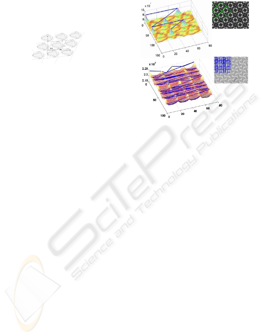
Several techniques have been employed to ap-
proach the 2D periodicity problem, as described in
detail in (O’Mara, 2002). The most common method
is autocorrelation. It is based in using part of the im-
age (typically one half) as a mask and performing
the autocorrelation of this mask with the whole im-
age. The peaks, or local maxima, of the autocorrela-
tion map can be extracted and the vectors that define
their unions used to propose a grid. Fig. 2 shows two
examples of autocorrelation maps on grey level im-
ages and the resulting grid superimposed on the im-
age from the point (0, 0). As may be noted, the sec-
ond case is wrong because the same threshold values
are used in both images and the correct tessellation is
not found. This example illustrates a common case of
autocorrelation failure. The threshold selection is an
image dependent problem, whereby images with low
dynamic range produce flat autocorrelation maps and
it is therefore difficult to find significant local max-
ima. In this work, we approach the problem in a dif-
ferent way. Instead of using the grey level values to
find the repetitiveness between image points, we use
a symmetries space whose values depend on the local
symmetries in the neighborhood of each image point.
Because wallpaper images have strong inherent sym-
metries, the values in this new space peak clearly and
are less dependent on the image contrast and noise.
Figure 2: Autocorrelation results on grey level images.
Left: autocorrelation peaks. Right: grid obtained from con-
necting a fixed number of peaks, as a ratio of the maximum.
The symmetries space is obtained through the
analysis of phase discrepancy (or congruency) be-
tween local frequency components at each image
point. These frequency components are computed at
several orientations and scales using wavelet filters.
This phase analysis enables the automatic detection
of these locally oriented symmetries and, therefore,
computes a high value of entropy, or symmetry, when
it estimates the orientation and scale corresponding
to the lengths or distances of appearing symmetries.
If more local symmetries appear at different orienta-
tions with the same periodicity value, then confidence
in that value increases. In short, this process obtains
the periodicity of the signal from the identification of
two local symmetries that repetitively appear in this
new space.
2 PHASE ANALYSIS
The chosen method of phase analysis was developed
by Kovesi (Kovesi, 1997). He established that im-
age features such as step edges, lines, roof edges and
match bands, all give rise to points where the Fourier
components of the image, computed at those points,
are maximally in phase. Oppositely, highly symmet-
ric image points will have minimally in phase fre-
quency components. Therefore, he introduces two
dimensionless quantities, called Phase Congruency
(PC) and Symmetry (Sym), which provide absolute
measurements of the significance of these feature
points. The use of phase congruency for marking fea-
LATTICE EXTRACTION BASED ON SYMMETRY ANALYSIS
397
tures has significant advantages over gradient based
methods. It is invariant to changes in image bright-
ness and contrast. Moreover it does not require any
prior recognition or segmentation of objects, thus en-
abling the use of universal thresholds values that can
be applied over a wide range of images.
Kovesi proposes a method to obtain these features,
based on the determination of the energy at a local
level. Kovesi’s method uses a multiresolution ap-
proach based on a pair of symmetric/antisymmetric
logGabor wavelet filters (M
e
, M
o
), from which an ac-
cumulated response for a given scale s and orientation
o is obtained using the eq. 1.
[e f
s,o
(x), o f
s,o
(x)] ← [I(x) ∗ M
e
s,o
, I(x)M
o
s,o
] (1)
The values e f
s,o
(x) (even) and o f
s,o
(x) (odd) can
be thought of as the real and imaginary parts of com-
plex valued frequency components. These values en-
able the content of a grey image to be rewritten as the
combination of a phase component (A
s
) and an orien-
tation component (φ) computed as follows:
A
s,o
(x) =
q
e f
2
s,o
(x) + o f
2
s,o
(x)
φ
s,o
(x) = atan2(e f
2
s,o
(x) + o f
2
s,o
(x))
(2)
The Symmetry measurement is computed through
the eq. 3. It provides a value of local symmetry com-
bining the phase and orientation components obtained
from filter responses over multiple scales and orienta-
tions, Sym(x), as:
∑
O
o=1
∑
S
s=1
cA
s,o
(x)[|cos(φ
o
(x)| − |sin(φ
o
(x)|] − T
o
c
∑
O
o=1
∑
S
s=1
A
s,o
(x) + ε
(3)
being φ(x) the overall mean phase angle, T
o
is a noise
compensation term that represents the expected re-
sponse from noise in the image (it is derived from the
computed values of A
o
=
∑
S
s=1
As, o), The ε is a small
constant to avoid ill-conditioned situations caused by
the very small values of the amplitude value A
s,o
. Eq.
3 can be rearranged as follow:
Sym(x) =
∑
O
o=1
∑
S
s=1
b[|e f
s,o
(x)| − |o f
s,o
(x)|] − T
o
c
∑
O
o=1
∑
S
s=1
A
s,o
(x) + ε
(4)
meaning that the symmetry value is the difference be-
tween the absolute responses of even-symmetric and
odd-symmetric wavelet filters. This measure varies
between [-1..+1] and is almost linear with phase devi-
ation. It must be noted that this model looks for image
transitions from white to black and in the reverse di-
rection. It can also be instructed to look for just one
transition by changing the term that involves the com-
bination of filter response. This is made by using a po-
larity parameter. Using the formulation for only one
transition (positive polarity) provides a wider range of
symmetry values, which facilitates the search for sim-
ilar values. Positive polarity is assumed in the rest of
the paper and the term −[e f
s,o
(x) − |o f
s,o
(x)|] is used
in the eq. 3. Thus, the Sym value ranges from [0.. +1].
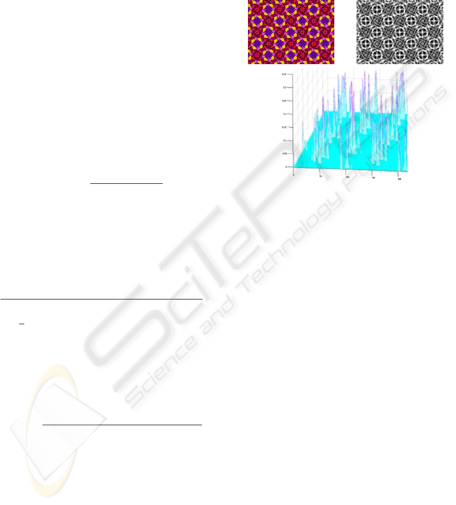
a) b)
c)
Figure 3: Kovesi’s phase analysis with polarity = +1: a)
original image, b) Symmetry values (equalized), and c) par-
tial 3D view of b).
Fig. 3 shows the results obtained applying eq. 4
over a grey level image (the luminance of the original
RGB image), with the default parameters proposed by
Kovesi. The motivation for making the transforma-
tion can be see in figure 3-c, where a detailed view of
the left part of the symmetry image is shown. It can
be seen that the transformation retains the repetitive-
ness and the spatial relationships of the original image
points, but it is now represented as peaks distributed
along the image in places where there is a high local
symmetry.
The phase analysis also produces, as a result, a
second component: the orientation component. This
reflects the orientation angle, for each image point,
for which the maximum symmetry value was reached.
We return to this component later.
3 LATTICE EXTRACTION
ALGORITHM
In this work we propose an methodology based on the
transformation from the bitmap space to a symmetry
domain where this search can be easily performed.
It is based on a three-stage algorithm to detect and
extract the grid of a regular image as follows: first,
transform from the original RGB values of image do-
VISAPP 2008 - International Conference on Computer Vision Theory and Applications
398

main into a symmetry domain (this is achived by us-
ing Kovesi’s symmetry model applied to a grey level
version of the original image); second, segmentation,
i.e. look for similar symmetry locations as identifiers
of equivalent local pixel contents; and third, detect
object unions by obtaining the direction vectors that
define the lattice by the studying the unions between
the identified observations.
The first step is made through the use of the phase
analysis to obtain symmetry values. The phase anal-
ysis is ran over a grey scale version (I: the luminance
component) of the original RGB image. The analysis
is repeated over a negative version of the image (∼ I)
to be able to cope with an initially unknown distribu-
tion of original pixel values, dark backgrounds, and
clear motifs, or viceversa. This results in two symme-
try images SymD (direct) and SymI (inverse), together
with their corresponding orientation images.
Some decisions about the parameters of this trans-
formation must be taken. Firstly, the number of lev-
els of the multiresolution analysis depend on the im-
age resolution, and goes from 1 to log
2
(max(M, N)),
MxN being the image size. Secondly, the number of
orientations (O) is initially chosen as 180 (the com-
plete range of directions on the plane [0..π[) by using
increments of 1 degree. Rotational symmetries lower
that 30 degrees are not allowed in wallpaper designs,
so a 7 degree step in orientations can be used with
sufficient accuracy - as the Nyquist theorem shows.
Finally, as the logGabor wavelet weighted by a
spread function is the filter used, the parameters of
both have to be chosen. For the wavelets, the cut-off
frequency value is computed from a minimum: the
minWaveLength value chosen as its related period can
be as much as the half the largest dimension of the
image, that is, to detect a minimum periodicity of 2 in
the image. For the spread that controls the sharpness
of the directional selectivity of the filters (as shown in
fig. 4 ), the orientation is used together with a con-
stant (dThetaOnSigma = 1.7) value that ensures an
even coverage of the 2-D frequency spectrum. The
combined response of the filters for a constant value
of frequency and spread value, but different values of
orientation can be seen in fig. 4.
At this point, the two versions (direct and inverse)
of the transformed domain of representation must be
examined and/or combined to obtain a binarized in-
termediate image - from which the last step can be
applied. This segmentation and direction determina-
tion needs a little more consideration if they are to be
achieved without imposing predetermined thresholds.
The subsections below discuss this topic.
Figure 4: From the left: filter appearance for a fixed value of
frequency, orientation of 0 and spread values of 0.5, and 1.0,
and examples of filter directionality, for a spread of 1,77, a
constant frequency value and orientations of 60, and 180
degrees.
3.1 Segmentation Step: Looking for
Objects
At this point, the two versions (direct and inverse) of
the transformed domain of representation must be ex-
amined and/or combined to obtain a binarized inter-
mediate image - from which the last step can be ap-
plied.
This stage consist in analysing each one of the
symmetry images by looking for points that exhibit
the same maximum symmetry value. At least, three
are needed to establish two directions and, with them,
the resulting grid. But because we are working only
with the maximum values of the symmetry image, the
influence of noise is very marked. A more robust
strategy is possible by taking into account the neigh-
bourhood points of each local maximum because they
correspond to nearby points with high symmetry val-
ues.
To do this we perform a thresholding of the sym-
metry images with a iteratively decreasing threshold
value (T Sym) that is a percentage of the absolute max-
imum value. In each iteration, two binary images
(ob jectsD, ob jectI) are made showing “objects”, in
the sense of areas, around the local maxima that ap-
pear repeatedly and show certain shape regularity. A
simple labelling and comparison step enable us to ex-
tract these objects and obtaining the more frequently
repeated objects. A comparison measure between ob-
jects is taken as the euclidean distance between the
objects bounding boxes equalized and centered on the
mass center. As we do not know how much similar
the objects are, we use a threshold (T Similitude) that
is a percentage of the normalized euclidean distance.
This value is iteratively decreased until a minimum
number of similar objects is found. By putting this all
together we have the first version of the segmentation
algorithm as:
function [objs,nObjs]<-extractObjs(symD,symI)
TSym <- 100%;
while (nObjs < 4) and (TSym > 0)
objectsD <- threshold( SymD, TSym )
objectsI <- threshold( SymI, TSym )
TSimilitude <- 100%;
while (nObjs < 4) and (TSimilitude > 0)
LATTICE EXTRACTION BASED ON SYMMETRY ANALYSIS
399
objs, nObjs<-count & compare (objectsD,
objectsI, TSimilitude)
if (nObjs < 4)
TSimilitude <- TSimilitude - 1;
endIf
endWhile
if (nObjs < 4)
TSym <- TSym - 1
endIf
endWhile
endFunction
The algorithm progress until a minimum number
of objects (three) are found, or until the T
Sym
range
has been exhausted. For simplicity, error checking
and convergence tests have not been included. Seg-
mentation in the symmetry domain was still difficult
because of the existence of noise and strange values
obtained on the image border.
As an alternative, we studied the feasibility of the
orientation component that can be derived from the
phase analysis. We found that, in general, high values
in the symmetry domain were the result of the accu-
mulative contribution of filter responses over a wide
range of orientations. Furthermore, if we only look
in one orientation, a directly binarized version of the
orientation image can be obtained. In this image, a
value of 1 indicates that there was an “appreciable”
filter response in that direction, and a zero if not. The
decision about the appreciable filter response is based
on comparison with an estimation of the noise in each
image. These values are computed from the symme-
try value of the minimum analysis scale.
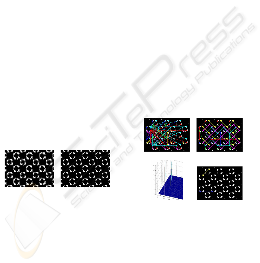
a) b)
Figure 5: Segmentation stage can be conducted over (a)
symmetry (equalized) or (b) orientation components.
We found that this binary orientation image re-
flects the same objects as those found around the lo-
cal maxima in the symmetry space. Fig. 5 shows this
idea. In this work, we propose the use of this binary
orientation component because it is easier, than the
symmetry component, as thresholds do not have to be
established to segment objects. We propose a second
version of the segmentation algorithm as follows:
function [objs, nObjs]<-extractObjs(
orientacionD, orientacionI )
objectsD <- orientacionD
objectsI <- orientacionI
TSimilitude <- 100%;
while (nObjs < 4) and (TSimilitude > 0)
objs, nObjs<-count & compare (objectsD,
objectsI, TSimilitude)
if (nObjs < 4)
TSimilitude <- TSimilitude - 1;
endIf
endWhile
endFunction
3.2 Object Union Step
This point is devoted to the techniques that can be
used to establish the correct connection of the points
detected by the previous phase. They are focused on
the use of Hough and computational geometry tech-
niques. This is the same with any of the techniques
set forth in the introduction to solve the problem of
detecting periodicity.
Our proposal is to solve this stage in a three-step
filtering function. Firstly, to be consistent with the
definition of periodicity of a signal, we will restrict
the list to the connections that are ”observable” be-
tween recurrences of the same object in the image.
Two elements are considered equal (fig. 6-a)) if they
are similar in their characterization of “locally sym-
metrical”, i.e, the form of objects. This is the set of
possible directions.
a) b)
c) d)
Figure 6: Stages of the object union: (a) all possible con-
nections, (b) removing by grid restrictions, (c) voting re-
sults (number of votes for each orientation and displace-
ment pair), and (d) choosen directions.
Secondly, we reduce this connection list by using
the spatial constraints imposed by grid definition. Ac-
cordingly, a path between any of the grid points is
composed of a minimum number of minimum length
local connections. As described in (Mount, 2001),
this is the area of computational geometry. We use
the Relative Neighbourhood Graph (RNG) algorithm
over the established connections to obtain structurally
logical connections, because of its ability (Toussaint,
VISAPP 2008 - International Conference on Computer Vision Theory and Applications
400
1980), to extract a perceptually meaningful structure
from a set of points. Finally, in a last step we use a
voting scheme for the selected connections to choose
the two most repeated (fig. 6-c)). These two connec-
tions define the grid parameter (fig. 6-d)) and they
they define the grid geometry (fig. 6-d)) as shown onf
the next algorithm:
function [grid] <- vDirectors(objects, nObjs)
directionList <- tentativeGrid( objects )
directionList<-reduceConections( directionList )
v1,v2 <- vote( directionList )
grid <- (v1, v2)
endFunction
4 EXPERIMENTS
Once the lattice geometry has been extracted, a fi-
nal step is needed in order to evaluate the cor-
rectness of the method. To achive this, correct
databases together with a comparison method must
be established. “Wallpaper Groups” (Joyce, 1997),
“Wikipedia Wallpaper Groups page” (Wikipedia,
2007), “Basic Tilings” (Savard, 2001), and “PSU
Near-Regular Texture Database” (Lee, 2001) contain
some image collections closely related to the ones in
our field of application. An example of results ob-
tained with the first of these databases is shown in fig.
7. We have complemented the set by adding new im-
ages resulting from the application of a set of rigid
geometric transformations and different noise mod-
els in order to provide for wide range in the samples
available.
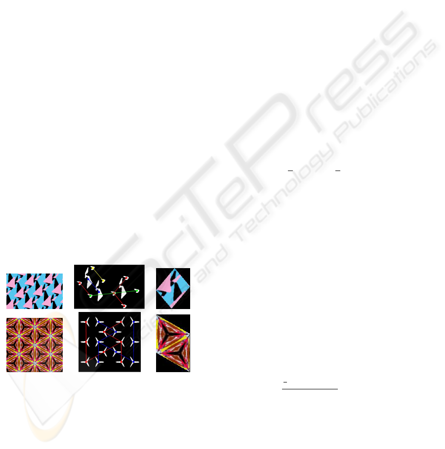
Figure 7: Results for some images (from left to right): orig-
inal image, established directions, and FP from image cen-
ter.
With respect to the comparison criteria, the lack
of uniformity and correct labeling of databases not
including grid geometry, makes expert intervention
sometimes necessary to evaluate the quality of the re-
sult. Nevertheless, an effort to define automatic cri-
teria based only on image parameters must be carried
out.
A first approximation is to define the error in
terms of the euclidean distance between the origi-
nal and a reconstructed image replicating a selected
FP obtained using grid parameters. Thus we define,
for example, the Mean FP (MNFP) and Median FP
(MDFP) as the parallelogram obtained, respectively,
through the mean or median of image pixels related
to the grid geometry extracted. The choice of the
representative parallelogram is important for the fi-
nal result of the reconstruction process, so it is not a
good statistical. Nevertheless, this method has sev-
eral problems: the selection of a representative FP
is needed, influencing the final statistical results; the
image comparison process not only evaluates the cor-
rectness of grid geometry but also evaluates the image
content; and the lack of measure normalization.
To solve these problems we propose to calculate
a measure of Grid Adjust Error (GAE) to quantify
the error between the grid geometry computed and
the true image geometry. The formulation is done us-
ing a geometrical criteria intended to minimise errors
related to pixel distribution over the image, as char-
acterized by its variance S
2
, which can be expressed
as:
S
2
=
1
n
r
∑
i=1
n
i
S
2
i
+
1
n
r
∑
i=1
n
i
( ¯x
i
− ¯x)
2
(5)
Where the image has been divided in r sets of size
n
i
, mean ¯x
i
and variance S
i
, being n the size of the
image, n = n
1
+ n
2
+ ... + n
r
, and ¯x is the mean.
We use an image partition based on the computed
grid geometry and define the Variance FP (V FP) in a
similar way to (MNFP) and (NDFP) but using pixel
variance instead of mean or median. Thus the terms
in eq. 5 are instanced as S
i
= V FP
i
and ¯x
i
= MNFP
i
.
In such a way, when the geometry of the lattice is cor-
rectly determined, the first term of equation tends to
zero and the second term to image variance. When
the computed geometry is incorrect, the opposite ef-
fect occurs. Both terms in eq. 5 range from 0 to S
2
.
Since we need to reduce image distribution ef-
fects, finally we propose the normalized measure of
GAE as follow:
GAE =
1
n
∑
r
i=1
n
i
V FP
i
S
2
0 6 GAE 6 1 (6)
Experiments with a number of 100 random lattices
were attempted on the wallpaper set, with the aim
of showing the statistical value tendency for wrong
lattices. The obtained variance values are between
553, 28 and 9804, 8, the statistic produced a mean
value of between 0, 945 and 1, 019, while the standard
deviation of the values is between 0, 008 and 0, 119.
The observed mean values over one are inherent in the
process of quantization: a result of the maths errors on
LATTICE EXTRACTION BASED ON SYMMETRY ANALYSIS
401

Table 1: Lattice evaluation for some images in Wallpaper
database.
GAE
nok
I S
2
V FP
ok
GAE
ok
[m, σ]
1 6070,0 529,7 0,09 [0,98, 0,08]
3 7564,4 1722,9 0,23 [0,94, 0,16]
4 6574,3 1581,7 0,24 [0,99, 0,04]
7 2538,3 619,3 0,24 [1,01, 0,02]
8 553,3 137,3 0,25 [1,00, 0,03]
9 7052,3 2258,6 0,32 [1,01, 0,07]
10 3218,9 946,7 0,29 [0,98, 0,19]
13 1115,6 380,5 0,34 [0,95, 0,17]
17 5511,6 2300,4 0,42 [0,95, 0,15]
rounding the values of the computed lattice geometry
to obtain pixel coordinates of the image.
Results for the “Wallpaper Groups” database are
shown in table 1. This table shows, from left to right,
image numbers and variance: the highness of this
value means that there is a greater dispersion on pixel
values; in regular images (as is the case) this means
there is noise. The next columns are the weighted
means of V FP and, the GAE values for the correct
grid extracted for the current image. Finally, a sta-
tistical distribution of GAE appears when using grids
extracted from the rest of the images, and this means
wrong lattice geometry values. From the last two
columns, as it was observed in the other collections,
the values of the statistical near to 0 identify a correct
lattice, meanwhile when this value is very near to 1
(the greatest deviation is 0, 19) can be concluded that
the lattice used does not offer a good reconstruction,
and it does not explain the image content.
5 CONCLUSIONS AND FUTURE
WORK
This work has shown an approach for extracting lat-
tice in regular image based on phase analysis. To
achive this goal we have revised the literature, and
observed the existing problems. The correspondence
between a formulation of lattice based on periodicity
versus symmetry, has led us to examine a multireso-
lution wavelet transform implementation. The study
of this, together with the justification of how to cal-
culate the parameters of the proposed technique, has
resulted in an algorithms that produces a process that
can auto-adjust itself to the circumstances of each im-
age. A set of experiments was conducted on this al-
gorithm, and the results in the determination of the
lattice have been applied to different sets of images.
In addition, as products of this work, an statistic
is proposed to evaluate the correctness of the algo-
rithm. A methodology is also proposed that cover
all the variations an image may undergo, typically in
the context proposed for implementation. As lines of
future work we plan to explore: (a) the computation
of the rest of isometries that help us choose to which
Plane Symmetry Group an image belongs; (b) to ob-
tain a statistical confirmation of the behaviour of the
GAE values for geometry values nearby to those of
the correct lattice; and (c) extract all the information
from the symmetry component, starting from the idea
that this aspect leads us to detect directly the axes of
reflection symmetry present in the image.
As a practical demonstration of the use of the al-
gorithms submitted, we are using this technique of de-
tecting repetitive patterns for real situations such as:
(a) obtaining a structural representation or syntactic of
the image that can be used for CBIR, and (b) rebuild-
ing, or recovering, the contents of an image, that has
been spoiled by noise, because stains, holes, breaks,
and other defects that involve the breakage or incom-
pleteness of the image.
ACKNOWLEDGEMENTS
This work is supported in part by project VISTAC
(DPI2007-66596-C02-01).
REFERENCES
Horne, C. E. (2000). Geometric symmetry in patterns and
tilings. Woodhead Publishing. ISBN 1 85573 492 3,
Abington Hall (England).
Joyce, D. E. (1997). Wallpaper groups (plane symmetry
groups). http://www.clarku.edu/ djoyce/.
Kovesi, P. (1997). Symmetry and asymmetry from local
phase. In AI’97, Tenth Australian Joint Conference on
Artificial Intelligence. pp 185-190.
Lee, S. (2001). Psu near-regular texture database.
http://vivid.cse.psu.edu/texturedb/gallery/.
Mount, D. (2001). Computational geometry: Proximity and
Location, cap. 63. CRC Press, 0-8493-8597-0.
O’Mara, D. (2002). Automated facial metrology, Chapter
4: Symmetry detection and measurement. PhD thesis,
University of Western Australia.
Savard, J. J. G. (2001). Basic tilings: The 17 wallpaper
groups. http://www.quadibloc.com/math/tilint.htm.
Toussaint, G. T. (1980). The relative neighbourhood graph
of a finite planar set. Pattern Recognition, vol. 12, pp.
261-268.
Wikipedia (2007). Wallpaper group — wikipedia, the free
encyclopedia. http://www.wikipedia.org/.
VISAPP 2008 - International Conference on Computer Vision Theory and Applications
402
