
CHARA
CTERISATION AND AUTOMATIC DETECTION OF LYMPH
NODES ON MR COLORECTAL IMAGES
Jeong-Gyoo Kim and J. Michael Brady
Dept. Engineering Science, Oxford University, Parks Road, Oxford, UK
Keywords:
Medical image analysis, lymph node characterisation, PDF modelling, and segmentation.
Abstract:
Colorectal cancer is the second most common cause of death in Western countries. It is often curable by
chemoradiotherapy and/or surgery; however, accurate staging has a significant impact on patient management
and outcome. Numerous clinical reports attest to the fact that staging is not currently satisfactory, and so
more precise methods are required for effective treatment. The three major components of disease staging are
tumour size; whether or not there is distal metastatic spread; and the extent of lymph node involvement. Of
these, the latter is currently by far the hardest to quantify, and it is the subject of this paper. Lymph nodes are
distributed throughout the mesorectal fascia that envelops the colorectum. In practice, they are detected and
assessed by clinicians using properties such as their size and shape. We are not aware of any previous image
analysis approach for colorectal images that makes this subjective approach more scientific.
To aid precise staging and surgery, we have developed methods that characterises lymph nodes by extracting
implicit properties as computed from magnetic resonance colorectal images. We first learn the probability
density function (PDF) of the intensities of the mesorectal fascia and find that it closely approximates a Gaus-
sian distribution. The parameters of a Gaussian, fitted to the PDF, were estimated and the mean intensity of
a lymph node candidate was compared with it. The fitting provides an explicit criterion for a region to be
classed as a lymph node: namely, it is an outlier of the Gaussian distribution.
As a key part of this process, we need to segment the boundaries of the mesorectal fascia, which is enclosed
by two closed contours. Clinicians recognise the outer contour as thin edges. Since the thin edges are often
ambiguous and disconnected, differentiating them from neighbouring tissues is a non-trivial problem; the
surrounding tissues have no significant difference from the mesorectal fascia in both intensity and texture. We
employed a level set method to segment three sets of objects: the mesorectal fascia, the colorectum, and lymph
node candidates. Our segmentation results led us to build a PDF and to use it for the criterion that we propose.
The whole process of implementation of our methods is automatic including the lookup of lymph candidates.
The results of clinical cases are summarised in the paper.
1 INTRODUCTION
Colorectal cancer is the second most common cause
of death in Western countries (McArdle et al., 2000)
and its incidence has increased in many Asian coun-
tries over the past few decades (Sung et al., 2005).
It is known that the disease is curable by chemora-
diotherapy and/or surgery if it is detected at an early
stage and treated appropriately; surgery is currently
the best curative therapy. Therefore, cancer staging
1
has a significant impact on patient management, not
least the decision whether to proceed to surgery.
1
The
extent to which a (colorectal) cancer has spread is
described as its stage.
Though accurate preoperative staging is essen-
tial for planning of optimal therapy, there have been
numerous clinical reports which attest to the fact
that preoperative staging accuracy based on clinician
judgement of images is not satisfactory (Filippone
et al., 2004), and so a method for more precise stag-
ing is required for patient management and effective
treatment. Staging of the disease is based on the TNM
classification: tumour size (T); whether or not there is
distal metastatic spread (M); and the extent of lymph
node involvement (N). Of these, the latter is currently
by far the hardest to quantify, and it is the subject of
this paper.
Lymph is a clear fluid that travels through the
body’s arteries, circulates through the tissues to
403
Kim J. and Brady J. (2008).
CHARACTERISATION AND AUTOMATIC DETECTION OF LYMPH NODES ON MR COLORECTAL IMAGES.
In Proceedings of the Third International Conference on Computer Vision Theory and Applications, pages 403-412
DOI: 10.5220/0001086204030412
Copyright
c
SciTePress

cleanse them and keep them firm, and then drains
away through the lymphatic system. Cancer cells
may drain into nearby lymph nodes, which are bean-
shaped structures that help fight against infection.
Lymph nodes are the filters along the lymphatic sys-
tem. Since the lymph nodes function to filter out
harmful cells, in particular cancer cells, this is a log-
ical place to look for cancer cells that have escaped
the original tumor and are seeking to metastasise to a
distal location. Lymph node dissection prevents can-
cer cells from further growth. The number of involved
lymph nodes strongly predicts the nature of the cancer
and the type of treatment needed to fight it. For these
reasons, it is considered by clinicians to be of great
importance to assess lymph nodes in the management
of cancer.
In the case of colorectal cancer, the lymph nodes
appear as dark small blobs on magnetic resonance
(MR) images and are distributed mostly in the
mesorectum, a fatty tissue that envelops the colorec-
tum. In practice, lymph nodes are characterised by
human vision using explicit properties, such as size
and shape of lymph nodes. We are not aware of any
method of image analysis approach of colorectal im-
ages that makes this subjective approach more scien-
tific.
In this paper we develop methods to aid precise
staging and estimation of the circumferential resec-
tion margin of colorectal cancers, namely detection
and characterisation of a lymph node. The contribu-
tion of the proposed methods can be divided into two
categories: modeling an intensity probability density
function (PDF) and segmentation of non-trivial MR
images.
Section 2 describes the methods we propose; char-
acterising a lymph node by building a PDF of inten-
sity of the mesorectal fascia. For this purpose, we
need to segment the mesorectal fascia on non-trivial
images as well as lymph node candidates. Our ex-
periments are presented in section 3, and section 4
concludes and discusses our work.
2 METHODS
Our methods include lymph node detection and char-
acterisation; the two unrelated categories are com-
bined here.
We attempt to detect and analyse lymph nodes
from 3D MR colorectal images, taken at our lo-
cal hospitals by GE 1.5T magnetic resonance imag-
ing scanners with parameters of TE = 120ms, TR =
6500ms. Each 3D dataset comprises a set of 23 to 30
slices each corresponding to a 3mm to 5mm slab of
tissue.
Lymph nodes generally appear as small dark
blobs, of a distinctively low intensity compared to
the surrounding fat which has high intensity. How-
ever, lymph nodes may be heterogeneous in intensity:
such heterogeneity is generally considered evidence
for a lymph node being affected by cancer. Further-
more, since lymph nodes are small and the sampling
in MRI is large compared to their size, the partial vol-
ume effect (PVE, in which multiple tissue structures
are present in a single voxel) has a substantial im-
pact on the intensities at locations that correspond to
lymph nodes. Also, the generally bright background
is punctuated with folds in the fat, which compli-
cate it appearance. The dark blobs corresponding to
lymph appear locally similar to blood vessels, espe-
cially when viewed in a single two dimensional slide
image. We can eliminate blood vessels on the basis of
their three dimensional shapes (extended over several
slices). The consecutive slices are registered and ex-
amined if they extend over several slices; if so, they
are more likely to be blood vessels. As a result, we
may estimate locations of some possible lymph node
candidates. For each candidate we test our methods
described in this section.
Current characterisations of lymph nodes stress ei-
ther their size and/or shape (Lee et al., 1984; Brown
et al., 2003; Bond, 2006). Such criteria are observa-
tions of explicit properties, as seen on images. We
aim to extract implicit properties of lymph nodes us-
ing image analysis techniques, and which can lead to
a higher precision of lymph node criteria.
Lymph nodes are distributed in a priori unpre-
dictable locations within the mesorectum. Because
they are small, subject to the PVE, and are in un-
predictable locations, we first determine information
about the surrounding mesorectum and use it to lo-
cate the lymph nodes. More precisely, we first model
the PDF of the mesorectum. However, to estimate the
mesorectum PDF we first need to isolate it from its
surrounding tissues.
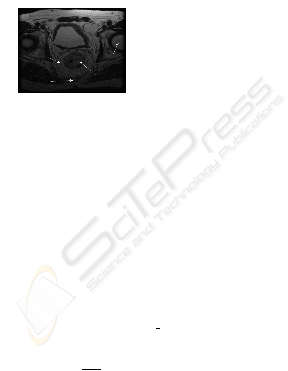
The dark round object at the lower center in Figure
1 is the colorectum. The object of higher intensity that
envelops the colorectum is the mesorectum, bound by
the mesorectal fascia. The mesorectal fascia can be
recognised by human vision as a very thin low signal
intensity, however, because of the low signal to noise
and the poor sampling density, edge detectors tend to
produce disconnected edges.
To isolate the mesorectum, we need to delineate
the boundary of the mesorectal fascia and the bound-
ary of the colorectum. The difficulty of this segmenta-
tion task derives from the fact that there is, in several
places, no intensity or texture difference between the
VISAPP 2008 - International Conference on Computer Vision Theory and Applications
404
50 100 150 200 250
50
100
150
200
250
mesorectum
femoral head
(hip bone)
colorectum
coccyx
bladder
Figure 1: A slice of an MR colorectal image: off-plane axial
view.
mesorectal fascia and surrounding tissues along the
thin edges. The shape of the mesorectal fascia varies
from patient to patient, as do the slice locations of the
patient.
Subsection 2.1 presents how we characterise
lymph nodes, while subsection 2.2 presents delin-
eation of the mesorectum and lymph nodes using level
set methods. The criteria on an automatic lookup of
lymph candidates are discussed in 2.3.
2.1 Characterisation of Lymph Nodes
As explained earlier, we try to extract implicit prop-
erties of lymph nodes that can be read from images.
The most common way of extracting a property of
image could be its intensity. We have examined sim-
ple statistics of the intensity of the mesorectum such
as moments: mean, variance, skewness and Kurtosis.
We found that such statistics are inadequate to differ-
entiate lymph nodes from the mesorectum.
For this reason, we first learn the intensity prob-
ability distribution function (PDF) of the mesorec-
tal fascia. This PDF is likely to be Gaussian as has
been frequently noted, for example (Cremers, 2006).
We have found that the PDF closely approximates a
Gaussian distribution N(µ,σ
2
). We also tested the
Rayleigh distribution (since this is ideally the noise
model for MRI), but we found that it was not as good
a fit to the intensity histogram as a Gaussian. The pa-
rameters µ and σ
2
of the Gaussian distribution vary
from patient to patient, so they should be estimated
for each individual.
We model the PDF with
P (x) ≈ α exp{−
(x −µ)
2
2σ
} (1)
where exp{·} is an exponential function. This re-
quires the fitting of the three parameters
2
α, µ and
σ to the intensity histogram. The candidate lymph
nodes can be differentiated from the mesorectal fas-
cia using the PDF. We know a priori that the lymph
nodes are darker than fat voxels in the mesorectal fas-
cia and so their intensity will fall into a range on the
left tail of the Gaussian curve. We have found in
our experiments that the lymph nodes are clustered
around, or below, µ −2σ of the estimated Gaussian
curve in equation (1). That is, our criterion for finding
a candidate lymph node is that it should be an outlier
of the Gaussan estimated with equation (1).
To utilise this characterisation method, we need
to segment the boundaries of the mesorectum, as dis-
cussed in the next subsection.
2.2 Detection of Lymph Nodes
As shown in Figure 1, the edges of the inner con-
tour of the mesorectum, i.e., the boundary of the col-
orectum, is rather clear. However, the outer bound-
ary of the mesorectum, the mesorectal fascia is very
ambiguous. We have tested various methods to seg-
ment the the mesorectal fascia, such as the EM algo-
rithm, hidden Markov random measure fields (Mar-
roquin et al., 2003), phase congruency (Felsberg and
Sommer, 2001), and anisotropic diffusion (Perona
and Malik, 1990). All these methods have performed
well on other images such as brain images. How-
ever, they performed considerably less well on our
colorectal images, partly because of the poor signal
to noise and partly because of ambiguous boundaries.
We needed a method to segment extremely thin edges
and have found that level set methods had superior
performance to all the other methods of segmentation.
Level set methods are briefly introduced next.
2.2.1 Level Set Methods for Segmentation
There have been numerous papers on segmentation
using the level set methods in image analysis areas
2
The scale factor α is remained in our expression to ap-
proximate the PDF P since we do not normalise the Gaus-
sian, say G(α,µ,σ). When normalised (i.e. the area below
the Gaussian curve in the upper half plane is 1), it can be
expressed by two parameters G(µ,σ) with the scale factor
1
√
2πσ
. One can use any of the both expressions for op-
timisation. In order to find optimal parameters, we used
line search, which is based on the gradient of G(α,µ, σ),
and the partial derivatives
∂G
∂α
,
∂G
∂µ
and
∂G
∂σ
are computed.
Since the function G(α,µ,σ) is linear with respect to α and
σ appears only in exp(·), this separation of the scale fac-
tor makes
∂G(α,µ,σ)
∂σ
simpler than
∂G(µ,σ)
∂σ
which tends to be
easily perturbed by a small change of σ and optimisation is
prone to fail with.
CHARACTERISATION AND AUTOMATIC DETECTION OF LYMPH NODES ON MR COLORECTAL IMAGES
405

since the early work in the 90’s such as Malladi et al.
(Malladi et al., 1995) and Caselles et al. (Caselles
et al., 1997). One of the well known advantages of
such methods is that they are able to model topolog-
ical changes of boundaries of objects, merging and
splitting, during the evolution of an embedded func-
tion (Sethian, 1999).
Within the level set framework of Osher and
Sethian (Osher and Sethian, 1988), various types of
energy functionals are employed (Chan and Vese,
2001; Paragios and Deriche, 2000; Yezzi and Soatto,
2003; Li et al., 2005). Most researchers use a signed
distance function for an initial φ; but recently some
have suggested that the initial function does not have
to be a distance function. With alternative types of
initial functions such as piecewise constant functions,
Lee and Seo (Lee and Seo, 2006) and the work of D.
Cremers’s group have demonstrated successful imple-
mentations of level set methods.
We adopted the model proposed by Chan and Vese
(Chan and Vese, 2001), since it has shown superior
performance on our colorectal images to other level
set models. The model is not based on the image gra-
dient of the image to stop the process, but is based on
the segmentation techniques of Mumford-Shah func-
tional (Mumford and Shah, 1989). The fitting term
of the their energy functional is designed to be min-
imised when the segmented contour is on the bound-
ary of the object; the regualisation term is defined
by the area of the region inside the segmented con-
tour and its length. The model does not need to
smooth the raw image for segmentation, which is re-
quired in many other segmentation methods. When
smoothed, the very thin edges on our data sets were
buried into the surrounding tissues and this resulted in
poor performance of segmentation. The model gener-
ally copes well with the objects of ambiguous bound-
aries or reasonably noisy boundaries on images.
2.2.2 Segmentation of the Mesorectal Fascia
Chan and Vese (Chan and Vese, 2001) assume that the
intensity of an image can be approximated by a piece-
wise constant function u :
¯
Ω → R as do many other
segmentation techniques. In a simple case, a grey im-
age can be represented by a binary image, having two
values of intensity, and the locations (x,y) ∈ Ω where
there is a jump in the value of u occur will give a
segmentation result, a contour as the boundary of an
object.
A contour C ⊂ Ω is implicitly represented by the
zero level set of a Lipschitz function φ : Ω → R
in the level set method (Osher and Sethian, 1988);
C = {(x,y) ∈ Ω : φ(x,y) = 0}. The optimal contour
of the segmentation is attained by the evolution of the
embedding function φ(x,y,t) at time t and the pro-
cess amounts to solving a partial differential equation
(PDE) in the level set method;
∂φ
∂t
= 0.
Chan and Vese model an image as u(x,y) =
c
1
H(φ(x,y)) + c
2
{1 −H(φ(x,y))}, (x,y) ∈
¯
Ω, where
c
1
and c
2
are constants, and H is the Heaviside func-
tion. The constants c
1
and c
2
are in fact the average
values of intensity where φ ≥ 0 and φ < 0, respec-
tively.
To find an optimal piecewise constant function
to approximate the image, they evolve an embed-
ding function φ minimising the energy functional
F (c
1
,c
2
,φ) for appropriate parameters µ ≥ 0, λ
1
> 0
and λ
2
> 0;
F = µ
Z
Ω
δ(φ(x,y))|∇φ(x,y)|dxdy (2)
+ λ
1
Z
Ω
|u
0
(x,y) −c
1
|
2
H(φ(x,y))dxdy
+ λ
2
Z
Ω
|u
0
(x,y) −c
2
|
2
{1 −H(φ(x,y))}dxdy,
where δ is the 1D Dirac measure (as the weak deriva-
tive of H). The functional is a particular case of the
Mumford-Shah minimal partition problem (Mumford
and Shah, 1989). In order to solve the minimization
problem using variational calculus, we used the ap-
proximation H
ε
∈C
2
(
¯
Ω) of the Heaviside function H
and and its derivative δ
ε
in the energy function F as in
(Chan and Vese, 2001): H
ε
(z) =
1
2
(1 +
2
π
arctan(
z
ε
)),
δ
ε
(z) =
ε
π(ε
2
+z
2
)
. Note that lim
ε→0
H
ε
= H. The Euler-
Lagrange equation associated to the approximation to
equation (2) is led to
∂φ
∂t
= 0 in (0,∞) ×Ω, (3)
(IC) φ(0, x,y) = φ
0
(x,y) in Ω,
(BC)
δ
ε
(φ)
|∇φ|
∂φ
∂~n
= 0 on ∂Ω,
where ~n denotes the exterior normal to the boundary
∂Ω, and ∂φ/∂~n denotes the normal derivative of φ at
the boundary. The partial derivative in the PDE (3) is
∂φ
∂t
= δ
ε
(φ)
·
µdiv(
∇φ
|∇φ|
) −λ
1
(u −c
1
)
2
+ λ
2
(u −c
2
)
2
¸
.
The level set model with ε = 1 is used to segment the
mesorectum as well as candidates of lymph node.
2.3 Automatic 3D Lookup from 2D
Data Set
If the proposed methods are fully automatic, they
would be more practical. This subsection discusses
implementation criteria of automatic lookup to make
our methods fully automatic.
VISAPP 2008 - International Conference on Computer Vision Theory and Applications
406
The proposed methods of lymph node analysis can
be implemented with three stages: segmentation us-
ing a level set method, a lookup of candidates; analy-
sis of the candidates with a Gaussian estimate.
The level set method described in the previous
subsection is also used for delineation of lymph can-
didates on an image. The zero level set results in nu-
merous blobs on the image, and from them we must
select candidates of lymph nodes to analyse. The level
set implementation and Gaussian fitting proposed in
this section can be automatic. If we can make the
selection of candidates from the zero level set auto-
matic, the whole process will be fully automatic.
In section 2.1 we suggested intensity as a classi-
fication criterion of lymph nodes where Gaussian fit-
ting is utilised. There are other classification criteria
to be considered for lymph nodes and they will be in-
cluded in our automatic lookup stage.
In the clinical studies of lymph nodes (Brown
et al., 2003; Lee et al., 1984), large lymph nodes are
a sign of malignancy; 60% of involved lymph nodes
are 4mm diameter or larger in 2D images. We try to
look up even smaller blobs than this cilincal criterion
of size, which is based on human vision.
We look for candidates, 3D blobs, by reading 2D
images. Therefore, we need to consider connectivity
of 2D blobs between slices. For the connectivity, we
consider geometric structure of anatomy appeared on
2D image slices and provide a criterion of distance. If
a dark blob extends over a consecutive slice of thick-
ness 3mm and it runs at an extreme slope through
slices, it could be located as far as 8 pixel distance
on the consecutive slice of a 0.39mm ×0.39mm pixel
size; 4 pixel distance for a 0.78mm ×0.78mm pixel
size. Since patients remain still during an MR scan
and there is very little motion due to breathing, we
do not need to consider motion effect in the images.
Therefore, this geometric criterion is reasonable.
In the next section, the models summarised in this
section are implemented on MR images.
3 EXPERIMENTS
The images used in our experiments are T
2
weighted
MR colorectal images stored in DICOM format. They
are scanned off-plane and oblique axial thin section
as shown in Figure 1. Angulation of a scan plane per-
pendicular to the rectum is known in general to give
better information than other standard image planes
such as coronal and sagittal since the rectum is at an
angle. All images tested in this paper were scanned
either at John Radcliffe Hospital or Churchill Hospi-
tal, Oxford, UK. The parameters used in the 1.5T MR
scanner were TE = 120ms, TR = 6500ms, flip angle
= 90
◦
. Each slice of a sequence is taken at a uniform
distance.
Due to strong edges of neighbouring organs in
contrast to extremely thin edges of the mesorectal fas-
cia, we crop the images as in Figure 1 to a smaller
field of view than those shown in the left of Figure 2.
For our purposes, lymph node detection and char-
acterisation, we need to segment three objects from
images: the mesorectum, colorectum and a lymph
node candidate scattered in the mesorectum. Among
the various level set models that we have tested, such
as edge stopping, geodesic, and bandwidth, the model
of (Chan and Vese, 2001) showed better performance
on our images than other models. Their 2D model has
been found to be better than its 3D generalisation or
multi-phase model for our images.
slice 3
20 40 60 80 100 120
20
40
60
80
100
120
20 40 60 80 100 120
20
40
60
80
100
120
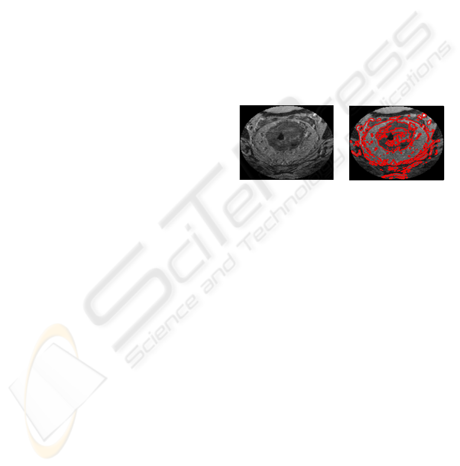
Figure 2: A small field of view MR slice(left); its segmen-
tation results of a level set method (right).
Subsection 3.1 presents the detection and charac-
terisation of a single candidate of lymph node. The
methods are extended to the automatic detection of
all possible candidates in subsection 3.2; a validation
issue is discussed in subsection 3.3.
3.1 A Single Candidate of Lymph Node
The first example set is presented in the left column
of Figure 3. The data set is a sequence of consec-
utive slices of 3mm thickness and the pixel size is
0.78mm ×0.78mm.
As described in section 2, we employed the model
of Chan and Vese and the resulting zero level set of an
optimal solution of the differential equation (3) was
obtained as presented in Figure 2 (right).
Then we organise the zero level set and selected
the contours delineating the three objects as presented
in the right column of Figure 3 at each corresponding
row. In the figures in the right column, the mesorec-
tum is delineated as the region enclosed by two closed
contours (red) for each of three images; the inner con-
tour is the boundary of the colorectum and the outer
contour the mesorectal fascia. A lymph node candi-
date is delineated by the green contour in the second
CHARACTERISATION AND AUTOMATIC DETECTION OF LYMPH NODES ON MR COLORECTAL IMAGES
407
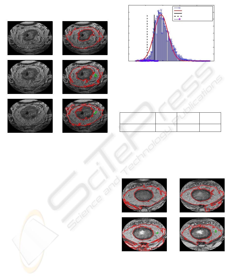
and third figure. In this case, as a result of our method,
an individual lymph node candidate is examined.
slice 1
20 40 60 80 100 120
20
40
60
80
100
120
slice1: 14 iterations
20 40 60 80 100 120
20
40
60
80
100
120
slice 2
20 40 60 80 100 120
20
40
60
80
100
120
slice2: 18 iterations
20 40 60 80 100 120
20
40
60
80
100
120
slice 3
20 40 60 80 100 120
20
40
60
80
100
120
slice3: 68 iterations
20 40 60 80 100 120
20
40
60
80
100
120
Figure 3: A set of consecutive MR slices with a small field
of view (left column); their corresponding mesorectal con-
tours selected from segmentation results by level set (right
column). Mesorectal contours and colorectal contours are
red, and a lymph node candidate green.
Our segmentation results enabled us to build a
PDF and to use it detect lymph nodes as outliers, as
described in section 2. We collect the intensity values
of the mesorectal fascia of the MR slices to learn its
voxel PDF. The voxel intensity histogram is depicted
in Figure 4 (blue stem and head). The optimal param-
eters of the Gaussian distribution are µ = 190.986 and
σ = 40.924. The optimal fit, with these parameters is
depicted by a red curve in Figure 4. Two vertical lines
for the values of µ −σ (solid line) and µ −2σ (dotted
line) on the horizontal axis are also plotted in the fig-
ure for the purpose of demonstration of our criterion.
Now we collect the intensity values of the lymph
candidate whose planar sections are depicted by green
contours in Figure 3. The histogram of the lymph
candidate (pink heads) is overlaid on the histogram of
the voxel intensity of the mesorectum, which appears
around the µ −2σ, at the left tail of the red Gaussian
curve in Figure 4. The mean intensity of the lymph
candidate is computed. The value is 118.709 and is
slightly larger than µ −2σ. These values are sum-
marised in Table 1 for comparison.
We have also tested datasets at a higher resolution,
i.e. images about four times bigger than the dataset
0 100 200 300 400 500
0
50
100
150
200
250
300
350
400
lymph candidate intensity and Gaussian fitting of MF intensity (3 slices)
intensity of MF (3 slices)
approximate Gaussian
µ − σ
µ − 2σ
lymph candidate
Figure 4: The histogram of the intensity of the mesorectum
of the three slices, delineated in Figure 3 (blue stem) and
its Gaussian estimate (red curve). The histogram of the in-
tensity of a lymph node candidate is overlaid (pink heads),
which is clustered around µ −2σ.
Table 1: Comparison of lymph node candidate to the pa-
rameters of Gaussian in Figure. 4
mean (lymph
candidate)
µ −2σ µ −1.5σ µ −σ
118.709 109.138 129.600 150.062
presented in Figure 3. The slice thickness of this ex-
ample set is 3mm and pixel size is 0.39mm ×0.39mm.
The four images are in Figure 5. The selected con-
tours from the segmentation results using the level set
method are presented in the figure.
slice1
50 100 150 200
20
40
60
80
100
120
140
160
180
200
220
slice2
50 100 150 200
20
40
60
80
100
120
140
160
180
200
220
slice3
50 100 150 200
20
40
60
80
100
120
140
160
180
200
220
slice4
50 100 150 200
20
40
60
80
100
120
140
160
180
200
220
Figure 5: A set of consecutive MR slices with a small field
of view and their mesorectal contours selected from seg-
mentation results by level set. Mesorectal contours and col-
orectal contours are red, and a lymph node candidate green.
The intensity of the segmented mesorectum of the
dataset is approximated by a Gaussian distribution in
Figure 6; the estimated parameters are µ = 336.906
and σ = 45.488. For this example, the mean intensity
VISAPP 2008 - International Conference on Computer Vision Theory and Applications
408

0 100 200 300 400 500 600 700
0
200
400
600
800
1000
1200
1400
1600
1800
lymph candidate intensity and Gaussian fitting of MF intensity (4 slices)
intensity of MF (4 slices)
approximate Gaussian
µ − σ
µ − 2σ
lymph candidate
Figure 6: The histogram of the intensity of the mesorectum
of the four slices, segmented in Figure 5 (blue stem) and its
Gaussian estimate (red curve). The histogram of the inten-
sity of a lymph candidate is overlaid (pink heads), which is
clustered below µ −2σ at the left tail of the Gaussian.
of the lymph node candidate seen in Figure 5 is com-
puted as 206.245. The comparison of the intensity
of the lymph node to the intensity of the mesorectal
fascia is given in Table 2. In this dataset, the mean
intensity of the lymph candidate is far smaller than
µ −2σ.
Table 2: Intensity comparison of lymph node candidate to
the parameters of Gaussian in Figure 6.
mean (lymph
candidate)
µ −2σ µ −σ
206.245 245.929 291.417
If we define the criterion of lymph node to be
smaller than µ −1.5σ, then the two individual can-
didates tested in this subsection are outliers of Gaus-
sians and are classified as lymph nodes.
3.2 Multiple Candidates of Lymph Node
We extend the methods for a single candidate pre-
sented in subsection 3.1 to all possible candidates.
In the first example set in subsection 3.1, we or-
ganised the zero level set to select possible candi-
dates from a few dozens to a hundred small blobs per
image. The candidates which are located within the
mesorectum and not very tiny are selected. Consider-
ing the criteria discussed in subsection 2.3, we set the
thresholds of the size of possible candidates and of
the distance for connectivity over slices. Our aim is
to provide more scientific methods and try to capture
small lymph nodes which can be missed by human vi-
sion. Hence, we select all blobs of 3mm diameter (i.e.
11 pixels of size 0.78mm×0.78mm) or larger and they
are candidates. The candidates are then analised with
their Gaussian estimates individually, as done in sec-
tion 3.1.
1st blob on slice 1
20 40 60 80 100 120
20
40
60
80
100
120
2nd blob on slice 1
20 40 60 80 100 120
20
40
60
80
100
120
Figure 7: Single blobs found as candidates (green).
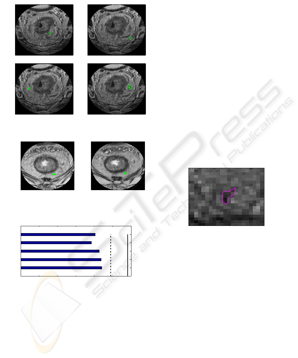
In this example of three slices, we selected 14 can-
didates from our lookup and some of them are pre-
sented in Figure 5 (appeared on consecutive slices in
the right column) and Figure 7 (appeared on a sin-
gle slice). The intensity of each candidate is grouped
and its mean intensity is computed. The mean inten-
sity values of these 14 candidates are plotted in the
horizontal bar chart in Figure 8. In the figure, seven
candidates are outliers of the Gaussian distribution in
Figure 4 and estimated as lymph nodes as suggested
in section 2. Some of the seven lymph nodes are de-
picted in Figure 9.
0 20 40 60 80 100 120 140 160 180
1
2
3
4
5
6
7
8
9
10
11
12
13
14
mean intensity of 14 lymph candidates
lymph candidates
intensity
µ − 2σ
µ −1.5σ
Figure 8: The mean intensity of detected candidates of the
three slices in Figure 3 are collected and their mean inten-
sity is plotted in the bar chart. Only seven candidates are
below µ −1.5σ of the Gaussian (solid vertical lines).
For the second example set in section 3.1, the
same procedure is carried out. In this example of four
slices, we selected five candidates; some of them are
shown in Figure 10 as well as Figure 5. The mean
intensity values of these five candidates are plotted in
the horizontal bar chart in Figure 11; all the candi-
dates are outliers of the Gaussian distribution in Fig-
ure 6 and estimated as lymph nodes.
We also tested a number of examples in which we
performed manual segmentation, In all these experi-
ments (of both automatic and manual segmentation),
CHARACTERISATION AND AUTOMATIC DETECTION OF LYMPH NODES ON MR COLORECTAL IMAGES
409
identified lymph node 1
20 40 60 80 100 120
20
40
60
80
100
120
identified lymph node 5
20 40 60 80 100 120
20
40
60
80
100
120
identified lymph node 6
20 40 60 80 100 120
20
40
60
80
100
120
identified lymph node 7
20 40 60 80 100 120
20
40
60
80
100
120
Figure 9: Candidates classified as lymph nodes (green).
4−th blob on slice 3
50 100 150 200
50
100
150
200
connected to 4−th blob on slice 4
50 100 150 200
50
100
150
200
Figure 10: Blobs selected as a candidate (green); connected
to consecutive slices.
0 50 100 150 200 250 300
1
2
3
4
5
mean intensities of 5 lymph candidates
lymph candidates
intensity
µ−2σ
µ−σ
Figure 11: The mean intensity of detected candidates of the
four slices in Figure 5 are collected and their mean intensity
is plotted in the bar chart. they are all below µ −2σ of the
Gaussian (dotted vertical lines).
the mean values of intensity of lymph candidates are
smaller than or slightly larger than µ −2σ. These ex-
periments enable us to ascertain that a mean value of
intensity is smaller than µ −2σ but for a population
set of a small size we need allow some margin of er-
ror in this criterion. For this reason, we suggest that
candidate lymph nodes correspond to being outliers
of the estimated Gaussian as
mean(lymph intensity) < µ −1.5σ
The estimation of the Gaussian of the mesorec-
tum enabled us to provide an explicit criterion for the
candidate to be classed as a lymph node. The whole
process of the proposed methods is fully automatic.
3.3 Manual Segmentation of Lymph
Candidates
We have compared our automatic method to manual
segmentation for the example set in Figure 9. We de-
tected five lymph nodes from our manually segmented
candidates using the same criteria as in the automatic
segmentation. Among the seven blobs classified as
lymph nodes with automatic segmentation, four were
also detected with manual segmentation. Note that
this disagreement is not only due to the quality of
automatic segmentation but due to the subjectivity of
segmenting small objects.
An example enlarged is presented in Figure 12
which shows the difficulty of manual segmentation of
a small object on a noisy image.
lymph − manual segmentation
42 44 46 48 50 52 54 56 58 60
88
90
92
94
96
98
100
102
104
106
Figure 12: A manually segmented lymph candidate on a
blurred image.
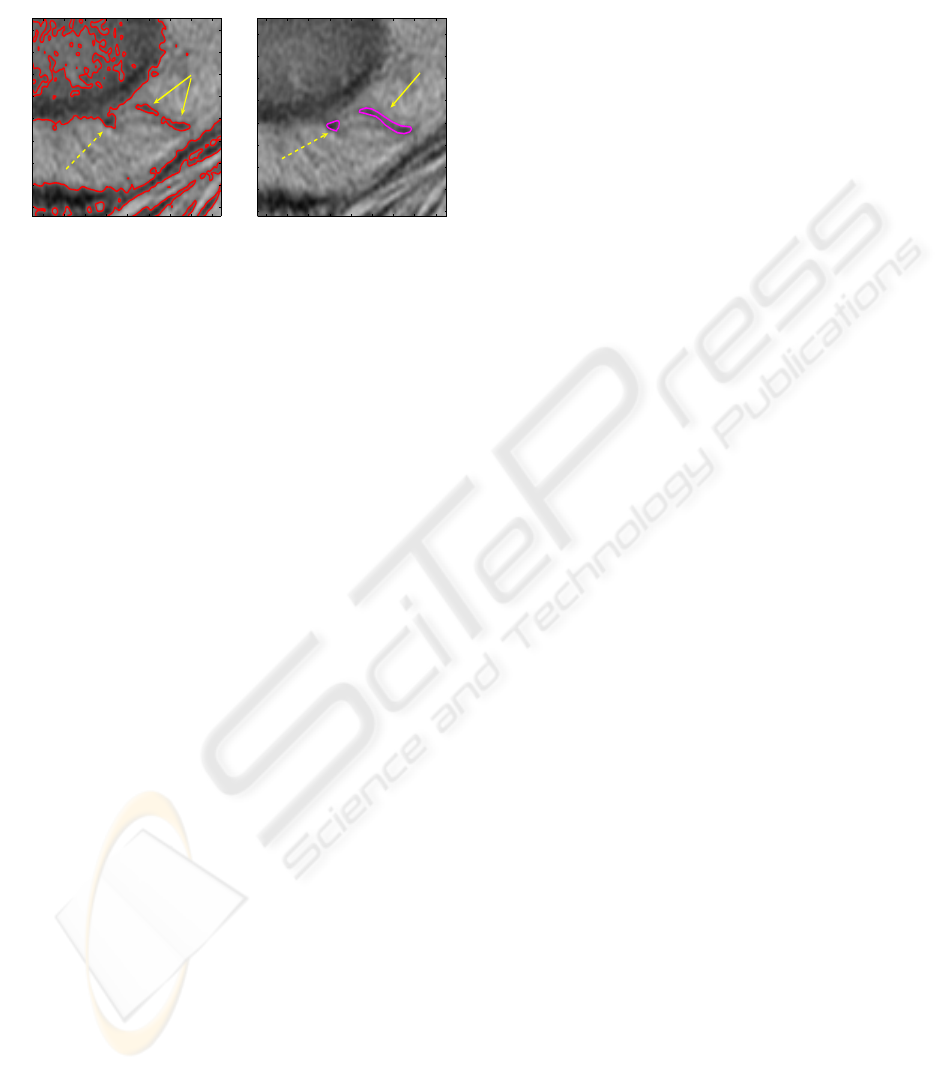
Another type of problems are demonstrated in
Figure 13; the figure on the left hand side was auto-
matically segmented, and the figure on the right hand
side was manually segmented. The figure demon-
strates the difference between machine vision (left)
vs. human vision (right) to segment lymph candi-
dates. The bump pointed by a broken arrow was
segmented into the region of colorectum with auto-
matic segmentation (left), but it was segmented man-
ually as a dark blob near the boundary of the col-
orectum (right). The other two dark blobs pointed by
solid arrows (left) were segmented automatically and
were included in the set of our candidates; while they
were merged into one object with manual segmenta-
tion (right), which can be classified as blood vessel
rather than a lymph node candidate. These are the
same problems as the current methods practiced by
clinicians, heavily relying on human vision. There-
fore, at this stage without further evidence, it is diffi-
cult to say if the three lymph nodes additionally de-
VISAPP 2008 - International Conference on Computer Vision Theory and Applications
410
tected by automatic segmentation and our charateri-
sation criterion are indeed false positives.
automatic segmentation
100 110 120 130 140 150 160 170 180
110
120
130
140
150
160
170
180
190
manual segmentation of lymph candidates
100 110 120 130 140 150 160 170 180
110
120
130
140
150
160
170
180
190
Figure 13: Differences between machine vision (left) vs.
human vision (right) in segmenting lymph node candidates.
Broken arrows: Part of the colorectum (left) or a blob
(right)? Solid arrows: two blobs (left) or blood vessel
(right)?
4 CONCLUDING REMARKS AND
DISCUSSIONS
We have proposed methods to characterise and detect
lymph nodes in MR colorectal images. Using a level
set method, we were able to delineate the boundaries
of the mesorctal fascia, colorectum, and a lymph node
candidate from non-trivial images. With the delin-
eated the boundaries, we estimated the intensity PDF
of the mesorectum, and approximated it by a Gaussian
distribution. The intensity of the segmented lymph
node candidate was then compared to the Gaussian
distribution. We suggest that lymph nodes can be de-
tected as outliers of the estimated Gaussian, with a
mean intensity smaller than µ −1.5σ. This provides a
more scientific means of lymph node characterisation.
The implementation is fully automated.
The number, size, and location of lymph node can-
didates on each slice vary. In our data sets, the thick-
ness of slice (usually from 3mm to 5mm) is quite large
in comparison to the pixel size (0.78mm ×0.78mm or
0.39mm×0.39mm). We cannot capture the true infor-
mation between slices and this may keep from precise
detection using information on images. For example,
learning the 3D connectivity of lymph candidates be-
tween 2D slices is not straightforward unless they are
sufficiently big. Since we implement a region merg-
ing algorithm individually for 2D slices and the slice
thickness is often larger than the lymph node size, a
high possibility of missing information exists. How-
ever, for small dark blobs that are prone to be missed
by human vision are able to be detected by the pro-
posed methods.
As discussed in subsection 3.3, validation is not
straightforward to carry out. Considering that pathol-
ogists routinely find more nodes in the dissected spec-
imen than reported by radiologists, a true validation of
a lymph node detection is very difficult.
Though better than the other segmentation meth-
ods examined, our level set implementation was not
always successful; leaking occurred when edges were
extremely thin and strong edges were nearby, as seen
in some slices in section 3.1 figures. Our character-
isation criterion of lymph nodes (Gaussian distribu-
tion thresholding) might not be sufficient. We think
our work is an initial study for more scientific meth-
ods of cancer staging and hope it promotes the active
study of lymph node detection using image analysis
approaches.
Some clinicians use signal heterogeneity as a
lymph characteristic. In our data sets, this was not
the case and thus we did not consider it in this pa-
per. However, for a large study population, this could
be taken into account in combination with the pro-
posed methods. Another plausible, yet highly in-
volved method may be to analyse the signal change
and heterogeneity of a lymph node where contrast
agent is used. These could be the subjects of our on-
going work.
ACKNOWLEDGEMENTS
This work was supported by GE.
REFERENCES
Bond, S. (2006). Image analysis for patient management
in colorectal cancer. PhD thesis, Oxford university,
Oxford, UK.
Brown, G., Richards, C., Bourn, M., Newcombe, R., Rad-
cliff, A., Dallimore, N., and Williams, G. (2003).
Morphological predictors of lymph node status in
rectal cancer with use of high-spatial-resolution mr
imaging with histopathologic comparison. Radiology,
227:372–377.
Caselles, V., Kimmel, R., and Sapiro, G. (1997). Geodesic
active contours. Int. J. Comp. Vis., 22:61–79.
Chan, T. and Vese, L. (2001). Active contours without
edges. IEEE Trans. on Image Processing, 10(2):266–
277.
Cremers, D. (2006). Dynamical statistical shape priors
for level set based tracking. IEEE Trans. PAMI,
28(8):1262–1273.
Felsberg, M. and Sommer, G. (2001). The monogenic sig-
nal. IEEE Transactions on Signal Processing, 49(12).
Filippone, A., Ambrosini, R., Fuschi, M., Marinelli, T.,
Genovesi, D., and Bonomo, L. (2004). Preoperative t
CHARACTERISATION AND AUTOMATIC DETECTION OF LYMPH NODES ON MR COLORECTAL IMAGES
411

and n staging of colorectal cancer. Radiology, 231:83–
90.
Lee, J., Heiken, J., Ling, D., Glazer, H., Balfe, D., Levitt,
R., Dixon, W., and Murphy, W. (1984). Magnetic
resonance imaging of abdominal and pelvic lym-
phadenopathy. Radiology, 153:181–188.
Lee, S. and Seo, J. (2006). Level set-based bimodal segmen-
tation with stationary global minimum. IEEE Trans.
on Image Processing, 15(9):2843–2852.
Li, C., Xu, C., Gui, C., and Fox, M. (2005). Level set evo-
lution without re-initialization: A new variational for-
mulation. In CVPR, pages 430–436.
Malladi, R., Sethian, J., and Vemuri, B. (1995). Shape
modeling with front propagation: a level set approach.
IEEE Trans. PAMI, 17(2):158–175.
Marroquin, J. L., Santana, E., and Bottelo, S. (2003). Hid-
den markov measure field models for image segmen-
tation. IEEE Trans. PAMI, 25(11):1380–1387.
McArdle, C., Kerr, D., and Boyle, P. (2000). Colorectal
Cancer. Isis medical Media Ltd.
Mumford, D. and Shah, J. (1989). Optimal approximation
by piecewise smooth functions and associated varia-
tional problems. Commun. Pure Appl. Math, 42:577–
685.
Osher, S. and Sethian, J. (1988). Front propagating
with curvature-dependent speed: algorithms based on
hamilton-jacobi formulation. J. Comput. Phys., pages
12–49.
Paragios, N. and Deriche, R. (2000). Geodesic active con-
tours and level sets for the detection and tracking of
moving objects. IEEE Trans. PAMI, 22(3):266–280.
Perona, P. and Malik, J. (1990). Scale-space and edge detec-
tion using anisotropic diffusion. IEEE Trans. PAMI,
12(7):629–639.
Sethian, J. (1999). Level Set Methods and Fast Marching
Methods: Evolving Interfaces in Computational Ge-
ometry,Fluid Mechanics, Computer Vision and Mate-
rials Science. Cambridge University Press.
Sung, J., Lau, J., Goh, K., and Leung, W. (2005). Increasing
incidence of colorectal cancer in asia: implications for
screening. The Lancet Oncology, 6(11):871–876.
Yezzi, A. and Soatto, S. (2003). Stereoscopic segmentation.
Int. J. of Comp. Vis., 53(1):31–43.
VISAPP 2008 - International Conference on Computer Vision Theory and Applications
412
