REPRESENTATION AND RECOGNITION OF HUMAN ACTIONS
A New Approach based on an Optimal Control Motor Model
Sumitra Ganesh and Ruzena Bajcsy
University of California, Berkeley, California, USA
Keywords:
Human Activity Recognition, Optimal Control, Multiple Model Estimation, Particle Filters.
Abstract:
We present a novel approach to the problem of representation and recognition of human actions, that uses an
optimal control based model to connect the high-level goals of a human subject to the low-level movement tra-
jectories captured by a computer vision system. These models quantify the high-level goals as a performance
criterion or cost function which the human sensorimotor system optimizes by picking the control strategy that
achieves the best possible performance. We show that the human body can be modeled as a hybrid linear
system that can operate in one of several possible modes, where each mode corresponds to a particular high-
level goal or cost function. The problem of action recognition, then is to infer the current mode of the system
from observations of the movement trajectory. We demonstrate our approach on 3D visual data of human arm
motion.
1 INTRODUCTION
The first fundamental problem in the analysis of hu-
man motion is that of representation. Several mod-
els of human motion have been proposed in literature.
In (Bregler and Malik, 1997), linear dynamical sys-
tems are used to model simple motions and high-level
complex motions are modeled using Hidden Markov
Models, where each state corresponds to a particu-
lar dynamical system. Layered structures of Hidden
Markov Models (Oliver et al., 2004)) and hierarchi-
cal Bayesian Networks ((Park and Aggarwal, 2004))
have been used to model multiple-levels of abstrac-
tion. The other broad approach has been to extract
3D spatio-temporal features or templates of move-
ments using Principal Component Analysis (PCA)
(Safonova et al., 2004), non-linear dimensionality re-
duction techniques (Fod et al., 2002) and other meth-
ods (Weinland et al., 2006).
In this paper, we propose a new approach to the
problem of representation based on an optimal control
model for human motion. The challenge lies in find-
ing a mathematical model that can connect the high-
level goals and intentions of a human subject to the
low-level movement details captured by a computer
vision system. Optimal control models of the hu-
man sensorimotor system do this in a natural manner.
These models quantify the high-level goals as a per-
formance criterion or cost function which the human
sensorimotor system optimizes by picking the control
strategy that achieves the best possible performance.
Thus optimal control models of human motion place
the high-level goals and the control strategy center
stage, while the movement details arise naturally as
a consequence of these goals. The different cost func-
tions (corresponding to different simple goal-directed
tasks), or equivalently the corresponding optimal con-
trol modules, are the basic building blocks in our rep-
resentation. We view the human motor system as a
hybrid system that switches between different control
modules, in response to changing high-level goals.
The problem of action recognition is to infer the hid-
den goal of the motion from observationsof the move-
ment trajectory. More complex actions can be mod-
eled as a composition of these basic goals. For ex-
ample, the action of lifting an object might be accom-
plished by the composition of two goal-directed mo-
tions - reaching for the object and then lifting it.
Optimal control models have been used in robotics
and computer animation ((Nori and Frezza, 2005),
(Li and Todorov, 2004)) for synthesis of motion,
and in the field of computational neuroscience as a
model for the human motor system. Optimal control
models of the human sensorimotor system ((Todorov,
2004), (Harris and Wolpert, 1998), (Scott, 2004))
have been successful in explaining several empirical
observations about human motion. Thus our model
is both theoretically justified and physically meaning-
99
Ganesh S. and Bajcsy R. (2008).
REPRESENTATION AND RECOGNITION OF HUMAN ACTIONS - A New Approach based on an Optimal Control Motor Model.
In Proceedings of the Third International Conference on Computer Vision Theory and Applications, pages 99-104
DOI: 10.5220/0001086700990104
Copyright
c
 SciTePress

ful. However, to the best of our knowledge, such a
model has not been used to analyze human motion or
recognize the higher-level goals of human motion.
Our approach is similar to (Bregler and Malik,
1997), in that we build our model using dynamical
building blocks or primitives, rather than purely kine-
matic ones (e.g. (Fod et al., 2002)). But while the
dynamical primitives in (Bregler and Malik, 1997) do
not model the forces or control input involved in pro-
ducing the motion, the control strategy plays a cen-
tral role in our representation. In (Del Vecchio et al.,
2003) Del Vecchio et al. used a switching linear dy-
namical system with simple control to study the 2D
motion of a computer mouse being used to draw fig-
ures. However, our control model is richer and we test
our hypotheses on 3D motions of the human arm.
The paper is organized as follows. In section 2 we
describe our model of the human motor system, with
particular emphasis on the control model. In section
3, we define the estimation problem and refer to the
methods we use. In section 4, we describe the experi-
mental setup and present results of the mode recogni-
tion on human arm data. We conclude by indicating
directions of future work and possible applications of
our work.
2 MODELS
In our model, the human motor system can be viewed
as a hybrid system that switches between different
control modules or modes as defined by the differ-
ent cost functions (goals). We assume here that the
cost functions corresponding to the different goals are
known to us. Given noisy kinematic observations of
a motion (e.g. the 3D hand trajectory for an arm mo-
tion), we wish to estimate the underlying mode se-
quence, or in other words, the sequence of basic un-
derlying goals that motivated the motion. To define
the problem more precisely we need to define models
for the following :
1. Mode Evolution : Since each mode corresponds
to a different goal, this model describes the prob-
ability of switching from one goal to another.
2. State Evolution : A biomechanical model is
needed to define how the control and the current
configuration/state of the body (joint angles and
velocities) determine the body configurationat the
next time instant.
3. Control : This model defines how the current state
and mode are used to arrive at a control input for
the biomechanical model.
4. Observation : The observation model defines the
relation between the joint angles and the observa-
tions.
We define these mathematical models and then
present the methods used for simultaneous state and
mode estimation from observations.
2.1 State Evolution Model
Let q(t) and τ(t) be n × 1 vectors (for n degrees of
freedom) that denote the joint angles and torques at
time t, respectively. The human body can be approxi-
mately modeled as a structure of rigid links connected
by joints. The equations of motion for such a model of
the human body are of the form (Murray et al., 1994)
M(q)¨q+C(q, ˙q)˙q+ N(q) = τ (1)
where the matrices M(.),C(.) and N(.) represent the
configuration dependent inertia, coriolis and gravita-
tional terms. Since M(q) is always positive definite,
this system can be feedback-linearized (Murray et al.,
1994) by designing the control torque to be of the
form
τ = M(q)u+C(q, ˙q)˙q+ N(q) (2)
where u is a control sequence. The equivalent lin-
earized system, from (1) and (2), is ¨q = u. By equiv-
alent what we mean is that optimal control methods
can be used to determine the form of the control u re-
quired for the ¨q = u system to achieve the goal. This
control u can then be transformed using (2) to obtain
the torques that need to be applied to the nonlinear
system in (1). This allows us to focus on the feed-
back linearized system as far as the mode estimation
is concerned. Also note that the linearized system is
independent of body parameters such as mass distri-
bution and length, which vary from subject to subject.
For a sampling period of ∆, the time-discretized
linear system of interest for the optimal control prob-
lem is
x
k+1
= Ax
k
+ Bu
k
+ v
k
(3)
where x
k
, the state at time k∆, is a 2n × 1 vector of
the joint angles and velocities at that time instant, v
k
is the process noise, u
k
is the control and
A =

I
n
∆I
n
0
n
∆I
n

(4)
B =

∆
2
2
I
n
∆I
n

2.2 Optimal Control
In this section we describe how the optimal control
law is determined for a general parametrized class of
VISAPP 2008 - International Conference on Computer Vision Theory and Applications
100

cost functions, when they are optimized for the lin-
earized state evolution model described in the previ-
ous section. The cost function we consider is of the
form
T
∑
k=1
(Cx
k
− r
k
)
T
Q
k
(Cx
k
− r
k
)
| {z }
accuracy
+
T−1
∑
k=1
u
T
k
Ru
k
| {z }
energy
+ ρT
|{z}
time
(5)
for a motion of duration T sampling instants. The pa-
rameters C,{r
1
,...r
T
},Q
k
≥ 0 can be used to specify
the goals or constraints, while the parameter R > 0 can
be used to specify the penalty on energy consump-
tion. The (Cx
k
− r
k
)
T
Q
k
(Cx
k
− r
k
) term constrains a
linear function of the state to be close to a reference
value r
k
. This term could be, for example, used to
impose the goal of reaching a certain configuration or
maintaining a certain pose by constraining the veloc-
ities to be close to zero. In the most extreme case,
we can specify an exact trajectory to be followed for
the entire duration. The last term imposes a penalty
on the duration of the motion. Thus, in minimizing
the cost function we attempt to achieve the goal with
minimum error, in the minimum time, while consum-
ing the least energy. The exact tradeoff between these
conflicting demands is determined by the cost func-
tion parameters Q
k
, R and ρ.
If the cost function only contained the first two
terms (accuracy and energy), the resulting optimal
control problem is called a Linear Quadratic (LQ)
problem. In the LQ problem the duration of the mo-
tion is fixed. The interesting thing about the solution
to this problem (see (Lewis and Syrmos, 1995) for de-
tails) is that not only is the form of the control known,
but the optimal cost-to-go, i.e. the minimum total cost
incurred from any time k until the fixed final time T,
can be computed as a function of the current state x
k
and the system parameters. Thus, given the current
state we can compute the minimum cost-to-go for dif-
ferent values of the final time T. Denoting the first
two terms of (5) as J
LQ
(), and the optimal cost-to-go
function as V(), the minimum value of the cost func-
tion in (5) can be written as
J
∗
= min
x
2:T
,u
1:T−1
,T
J
LQ
(x
2:T
,u
1:T−1
) + ρT (6)
= min
T
ρT + min
x
2:T
,u
1:T−1
J
LQ
(x
2:T
,u
1:T−1
)
= min
T
ρT +V(x
1
,T) .
The optimal time T
∗
can be obtained as T
∗
=
argmin
T
ρT +V(x
1
,T). The problem of minimizing
(5) then reduces to the LQ problem of minimizing the
first two terms for a fixed final time T = T
∗
.
Standard results from optimal control theory
(Lewis and Syrmos, 1995), can then be used to de-
termine the form of the control u
k
.
u
k
= −K
fb
k
x
k
+ K
ff
k
z
k+1
(7)
where the feedback and feedforward gain matrices,
K
fb
k
and K
ff
k
respectively, and the auxiliary sequence
z
k+1
are determined by a backward recursion that
is independent of the state sequence and only de-
pends on the system and cost function parameters
(See (Lewis and Syrmos, 1995) for details).
To summarize, the parameters of state evolution
model (3) and the cost function (5) completely deter-
mine the form of the optimal control u
k
as a function
of the current state x
k
. Thus, given the current mode
and state, the control input to be applied to optimize
the cost function corresponding to that mode (goal)
can be determined.
2.3 Mode Evolution and Observation
Models
The modes can be modeled as states of a markov
chain. Let m
k
, an integer value drawn from the set
{1,..,N}, represent the current mode i.e. which of
the N possible control modes is effective in determin-
ing the state transition from the (k − 1)-th sampling
instant to the k-th instant. The prior distribution of
modes is given by π
i
= P(m
0
= i), i = 1,. .., N and
the transition probabilities are given by
H
ij
= P(m
k
= j|m
k−1
= i) i, j = 1,.. .,N . (8)
The values of π
i
and H
ij
are assumed to be known.
The observations {y
1
,..., y
T
} available to us are of
the form
y
k
= g(x
k
) + n
k
, (9)
where the function g(.) and the distribution of the ob-
servation noise n
k
are assumed to be known.
3 STATE AND MODE
ESTIMATION
The recognition problem can be stated as follows :
given observations {y
1:T
} , {y
1
,..., y
T
} estimate the
state (joint angles and velocities) trajectory {x
1:T
},
the control sequence {u
1:T−1
} and the task or mode
trajectory {m
2:T
}. The problem requires simultane-
ous estimation of the continuous state and the mode
of the system. The control sequence is not an in-
dependent sequence - it is determined by the state
and the mode. Thus defined, the problem of action
recognition is one of mode estimation in a hybrid sys-
tem. Similar problems have been addressed in the
tracking of a maneouvering targets (McGinnity and
REPRESENTATION AND RECOGNITION OF HUMAN ACTIONS - A New Approach based on an Optimal Control
Motor Model
101

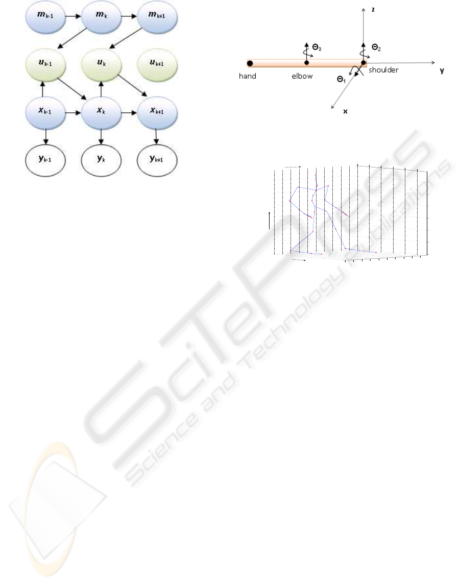
Figure 1: Graphical Model of State Evolution, Mode Evo-
lution, Control and Observations. The control is an inter-
mediate hidden variable that is completely specified by the
mode and the current state. Thus it is sufficient to estimate
the continuous state x
k
and the mode m
k
(hidden variables)
from the observations y
k
.
Irwin, 2000) and fault detection (de Freitas, 2002) in
systems. The Interacting Multiple Model (IMM) al-
gorithm (Blom and Bar-Shalom, 1988) and its vari-
ants (McGinnity and Irwin, 2000) have been the pre-
ferred method of solving this problem. We use a boot-
strap method similar to that in (McGinnity and Irwin,
2000), with an auxiliary particle filter (Pitt and Shep-
hard, 2001).
4 EXPERIMENTS AND RESULTS
We tested our ideas on 3D motion data sampled at 7
frames/sec, collected from a setup of 12 camera clus-
ters. We used the algorithm proposed by Lien et al.
in (Lien et al., 2007) for segmentation and tracking
of the joints of the body. Our test motions consisted
of motions of the arm for 2 subjects. The subjects
were instructed in two tasks that involved lifting a 5
lb weight. The tasks are shown in figure 4. Each
task consists of two goals, lifting and lowering, but
the manner in which these are to be accomplished is
different in the two tasks. Thus there are four distinct
goals or modes in the data set as shown in figure 4.
Five repetitions of each task were recorded for each
subject were used for testing.
For estimating the mode and state, we only use the
3D position trajectory of the hand with respect to the
shoulder as observations. The model of the arm and
joint angles are shown in figure 2, and the reference
coordinate system is shown in figure 3. The joint an-
gle values are specified with respect to the reference
Figure 2: Model of the arm.
0.5
1
1.5
2
2.5
3
0
2
4
6
8
10
12
−7
−6
−5
−4
−3
−2
−1
0
1
2
Z
Y
X
Figure 3: Coordinate System.
pose in figure 2, which corresponds to θ
1
= θ
2
= θ
3
=
0deg. The state of the system consists of the joint an-
gles and velocities i.e. x = [θ
1
θ
2
θ
3
˙
θ
1
˙
θ
2
˙
θ
3
]
T
. The ob-
servation function, that relates the joint angles to the
observations of the hand position, is given by
g(x) =


L
1
sin(θ
2
) + L
2
sin(θ
2
+ θ
3
)
−L
1
cos(θ
1
)cos(θ
2
) − L
2
cos(θ
1
)cos(θ
2
+ θ
3
)
−L
1
sin(θ
1
)cos(θ
2
) − L
2
sin(θ
1
)sin(θ
2
+ θ
3
)


(10)
where L
1
and L
2
denote the length of the upper and
lower arm, which are obtained from the segmentation
and tracking algorithm (Lien et al., 2007).
The cost functions for the four modes are con-
structed as follows. For modes 1 and 2, target poses
(r
T
) are specified in terms of constraints on θ
3
(θ
3
=
150 deg for mode 1 and 90 deg for mode 2) , the rota-
tion of the elbow joint. For modes 3 and 4, the target
poses are in terms of θ
1
(θ
1
= 0 deg for mode 3 and
90 deg for mode 4), the rotation of the shoulder joint
about the x axis. In all cases the final velocities are
constrained to be zero.
While the constraints arise naturally from our ex-
periment design and task specification, determining
the relative weighting of accuracy, energy and time
(Q,R,ρ) is not that simple. In this experiment we de-
termine these parameters by comparing simulations
with a training data set. We fixed Q
T
= 10
3
I
4
, and
R = 10
−3
I
3
for all modes. We found the value of ρ to
VISAPP 2008 - International Conference on Computer Vision Theory and Applications
102

be quite different for the two subjects - 100 for sub-
ject 1 and 25 for subject 2. This indicates that while
different subjects might have a common understand-
ing of the task definition, they might have different
preferences when it comes to the relative weighting
of accuracy, energy and time. These varying inter-
nal preferences might explain the stylistic variations
observed among subjects performing the same task.
This matter requires further study. In our experiment
we use different ρ values for the different subjects
during mode estimation.
Since the data set is fairly small, we set all the
modes to be equally likely apriori. The average time
spent in any mode τ, as observed in the training data
set, was used to set the transition probabilities as H
ii
=
1−(1/τ), i = 1,. ..N and H
ij
= (1−H
ii
)/(N−1)∀i 6=
j. The value of τ was fixed at 20 (sampling instants)
for the results below, but the estimation performance
was found to be not very sensitive to the value of τ.
The average accuracy of the mode estimation was
86 percent. The errors are almost entirely confined
to the segmentation boundaries as can be seen in fig-
ures 5 and 6. At other times, the mode is usually
correctly estimated with a high degree of confidence.
Figures 7 and 8 compare the estimated joint angles
with the ground truth obtained from the tracking al-
gorithm (Lien et al., 2007).
5 CONCLUSIONS
In this paper, we have proposed a new approach to
the problem of representation and recognition of hu-
man motion. Our experimental results clearly indi-
cate the validity of our proposal. However, there are
several issues that need to be addressed to solve the
action recognition problem comprehensively, within
this framework. Our experiments indicate that while
different subjects might share a common goal for the
motion, they might tend to tradeoff the competing
concerns of accuracy, energy and time differently. We
are currently working on extending the estimation al-
gorithm to estimate the relative weights online, along
with the state and the mode.
REFERENCES
Blom, H. A. P. and Bar-Shalom, Y. (1988). The interact-
ing multiple model algorithm for systems with marko-
vian switching coefficients. Automatic Control, IEEE
Transactions on, 33(8):780–783.
Bregler, C. and Malik, J. (1997). Learning and recognizing
human dynamics in video sequences. In IEEE Con-
ference on Computer Vision and Pattern Recognition
(CVPR), pages pp 568–674.
de Freitas, N. (2002). Rao-blackwellised particle filtering
for fault diagnosis. Aerospace Conference Proceed-
ings, 2002. IEEE, 4.
Del Vecchio, D., Murray, R., and Perona, P. (2003). Decom-
position of human motion into dynamics based primi-
tives with ap- plication to drawing tasks. Automatica,
39(12):2085–2098.
Fod, A., Matari´c, M., and Jenkins, O. (2002). Automated
Derivation of Primitives for Movement Classification.
Autonomous Robots, 12(1):39–54.
Harris, C. and Wolpert, D. (1998). Signal-dependent noise
determines motor planning. Nature, 394(6695):780–
4.
Lewis, F. and Syrmos, V. (1995). Optimal Control. Wiley-
Interscience.
Li, W. and Todorov, E. (2004). Iterative linear-quadratic
regulator design for nonlinear biological movement
systems. First International Conference on Informat-
ics in Control, Automation and Robotics, 1:222–229.
Lien, J.-M., Kurillo, G., and Bajcsy, R. (2007). Skeleton-
based data compression for multi-camera tele-
immersion system. In Proceedings of the Interna-
tional Symposium on Visual Computing, Lake Tahoe,
Nevada/California,Nov 2007, to appear.
McGinnity, S. and Irwin, G. (2000). Multiple model
bootstrap filter for maneuvering target tracking.
Aerospace and Electronic Systems, IEEE Transac-
tions on, 36(3):1006–1012.
Murray, R., Sastry, S., and Li, Z. (1994). A Mathematical
Introduction to Robotic Manipulation. CRC Press.
Nori, F. and Frezza, R. (2005). Control of a manipula-
tor with a minimum number of motion primitives.
Proceedings of the 2005 IEEE International Confer-
ence on Robotics and Automation, 2005., pages 2344–
2349.
Oliver, N., Garg, A., and Horvitz, E. (2004). Layered rep-
resentations for learning and inferring office activity
from multiple sensory channels. Computer Vision and
Image Understanding, 96(2):163–180.
Park, S. and Aggarwal, J. (2004). A hierarchical Bayesian
network for event recognition of human actions and
interactions. Multimedia Systems, 10(2):164–179.
Pitt, M. K. and Shephard, N. (2001). Auxiliary variable
based particle filters. In book Sequential Monte Carlo
Methods in Practice, Arnaud Doucet - Nando de Fre-
itas - Neil Gordon (eds). Springer-Verlag, 2001.
Safonova, A., Hodgins, J., and Pollard, N. (2004). Syn-
thesizing physically realistic human motion in low-
dimensional, behavior-specific spaces. ACM Trans-
actions on Graphics (TOG), 23(3):514–521.
Scott, S. (2004). Optimal feedback control and the neu-
ral basis of volitional motor control. Nature Reviews
Neuroscience, 5(7):532–546.
Todorov, E. (2004). Optimality principles in sensorimotor
control. Nature Neuroscience, 2004:907–915.
REPRESENTATION AND RECOGNITION OF HUMAN ACTIONS - A New Approach based on an Optimal Control
Motor Model
103

Weinland, D., Ronfard, R., and Boyer, E. (2006). Auto-
matic Discovery of Action Taxonomies from Multi-
ple Views. Proceedings of the 2006 IEEE Computer
Society Conference on Computer Vision and Pattern
Recognition-Volume 2, pages 1639–1645.
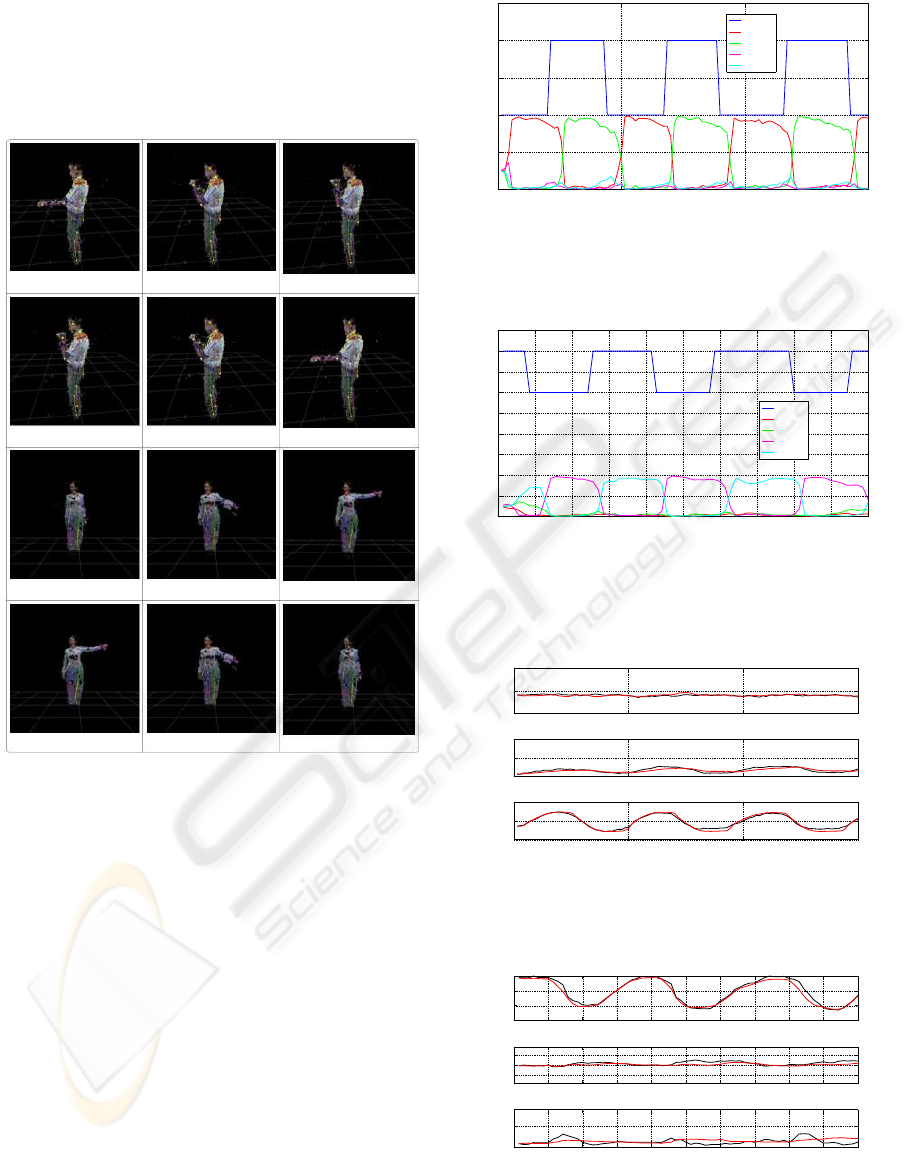
Figure 4: Modes in the Data. Row 1 : Task 1, Mode 1.
Row 2 : Task 1, Mode 2. Row 3 : Task 2, Mode 3. Row
4 : Task 2, Mode 4. In Task 1, the subjects lift and lower
the weights as indicated in rows 1 and 2, by only rotating
the elbow joint. In Task 2, the subjects lift and lower the
weights as indicated in rows 3 and 4, by only rotating the
shoulder joint about the x-axis.
0 5 10 15
0
0.5
1
1.5
2
2.5
sec
Mode
p(mode=1)
p(mode=2)
p(mode=3)
p(mode=4)
Figure 5: Mode Estimation : subject 2, task 1. In this task,
the mode switches between 1 and 2, as indicated by the blue
line. The other lines indicate the probability of each mode
at each instant.
0 1 2 3 4 5 6 7 8 9 10
0
0.5
1
1.5
2
2.5
3
3.5
4
4.5
sec
Mode
p(mode=1)
p(mode=2)
p(mode=3)
p(mode=4)
Figure 6: Mode Estimation : subject 1, task 2. In this task,
the mode switches between 3 and 4, as indicated by the blue
line. The other lines indicate the probability of each mode
at each instant.
0 5 10 15
0
100
200
θ
x
deg
0 5 10 15
0
100
200
θ
z
deg
0 5 10 15
0
100
200
θ
3
sec
deg
Figure 7: State Estimation : subject 2, task 1. Legend :
black line is the ground truth from the tracking algorithm,
red line is the estimate of the state.
0 1 2 3 4 5 6 7 8 9 10
−50
0
50
100
θ
x
deg
0 1 2 3 4 5 6 7 8 9 10
−50
0
50
θ
z
deg
0 1 2 3 4 5 6 7 8 9 10
0
100
θ
3
sec
deg
Figure 8: State Estimation : subject 1, task 2. Legend :
black line is the ground truth from the tracking algorithm,
red line is the estimate of the state.
VISAPP 2008 - International Conference on Computer Vision Theory and Applications
104