ITERATIVE RIGID BODY TRANSFORMATION ESTIMATION FOR
VISUAL 3-D OBJECT TRACKING
Micha Hersch, Thomas Reichert and Aude Billard
LASA Laboratory, EPFL, 1015 Lausanne, Switzerland
Keywords:
Stereo vision tracking, Rigid body transformation estimation.
Abstract:
We present a novel yet simple 3D stereo vision tracking algorithm which computes the position and orientation
of an object from the location of markers attached to the object. The novelty of this algorithm is that it does
not assume that the markers are tracked synchronously. This provides a higher robustness to the noise in the
data, missing points and outliers. The principle of the algorithm is to perform a simple gradient descent on
the rigid body transformation describing the object position and orientation. This is proved to converge to the
correct solution and is illustrated in a simple experimental setup involving two USB cameras.
1 INTRODUCTION
Estimating the 3-D rigid body transformation align-
ing two noisy sets of identifiable points is considered
a solved problem in computer vision. Indeed, various
closed form solutions have been suggested in the last
two decades (Arun et al., 1987; Horn, 1987; Walker
et al., 1991), and those solutions have been widely
used and compared (Eggert et al., 1997). However,
in spite of those existing solutions, we address once
again this problem and suggest an iterative solution to
the rigid body estimation problem. Our belief is that
in many applications, an iterative solution is prefer-
able to a closed-form solution, especially if the rigid
body transformation changes in time, for example
when tracking a moving object. The major reasons for
this is that an iterative solution would be more robust
to noise in the data and that and would not assume
synchronicity of the set of points.
2 SETTING AND NOTATIONS
We consider a rigid body transformation T transform-
ing a set of n vectors {x
i
} into another set of n vectors
{y
i
}. This transformation is described by a rotation R
around an axis passing through the origin and a trans-
lation V by a vector v:
y
i
= T(x
i
) = R(x
i
) + v. (1)
When considering a 3-D tracking application, the
rigid body transformation T can be used to describe
the position and orientation of the tracked object, rel-
atively to a reference position and orientation. The
reference positions of the n markers on the objects
make the set of {x
i
}. The positions of those mark-
ers when tracked by a stereo vision system constitute
the set of {y
i
}. It is assumed that the markers can be
distinguished one from another, for example by using
different colors. If the object is moving, the evolution
of T yields the trajectory of the object.
3 ROTATIONS
In this paper, we use the spinor representation of ro-
tations which is briefly recalled here, adopting the ap-
proach described in (Hestenes, 1999). This represen-
tation is very similar to the quaternion representation.
The spinor ¯q representing the rotation R is given by
a scalar α and imaginary vector bi. The direction of
b yields the rotation axis (passing through the origin)
and its norm is equal to sin(θ/2), where θ is the ro-
tation angle. The scalar α is given by cos(θ/2).The
rotation of a vector x by a spinor ¯q is given by the
following equation.
R
b
(x) = (1− 2b
T
b)x+ 2
q
(1− b
T
b)b× x+ 2(b
T
x)b,
(2)
where R
b
denotes the rotation represented by b.
674
Hersch M., Reichert T. and Aude A. (2008).
ITERATIVE RIGID BODY TRANSFORMATION ESTIMATION FOR VISUAL 3-D OBJECT TRACKING.
In Proceedings of the Third International Conference on Computer Vision Theory and Applications, pages 674-677
DOI: 10.5220/0001087106740677
Copyright
c
 SciTePress

4 ITERATIVE ESTIMATION OF A
RIGID BODY
TRANSFORMATION
We now present to the algorithm for iteratively esti-
mating a rigid body transformation given a set of n
points {x
i
} and its noisy transform {y
i
}. The princi-
ple of the algorithm is quite trivial. Starting from an
initial guess for the parameters b and v of the trans-
formation, it consists simply on a gradient descent on
the squared distance between the measurement y
i
and
the transformed point T
b,v
(x
i
)
∆b = −ε
∂
∂b
1
2






y
i
− T
b,v
(x
i
)






2
(3)
∆v = −ε
∂
∂v
1
2






y
i
− T
b,v
(x
i
)






2
, (4)
where ε is the learning rate. One assumes that i
takes values from 1 to n in a uniformly distributed
manner. So at each time step, an index i is selected
among the available points and b and v are update
according to (3) and (4).
The actual development of those two equations yields:
∆b = 2ε

y
i
− T
b,v
(x
i
)

T

− 2x
i
b
T
−
1
p
(1− b
T
b)
(b× x
i
)b
T
+ 1
q
(1− b
T
b)x
i
↑ +
bx
T
i
+ (b
T
x
i
)I

(5)
∆v = ε

y
i
− T
b,v
(x
i
)

, (6)
where I is the 3× 3 identity matrix and the unary
operator ↑ is defined as
x↑
.
=
∂
∂b
(b× x) =


0 x
(3)
−x
(2)
−x
(3)
0 x
(1)
x
(2)
−x
(1)
0


, (7)
with x = [x
(1)
x
(2)
x
(3)
]
T
.
This concludes the description of the algorithm.
For efficiency purposes, it is preferable to choose ref-
erence positions so that the x
i
are centered on the ori-
gin. This allows to reduce the influence of b on the
computation of v.
5 CONVERGENCE
In this section, we prove that if there exists a rigid
body transformation matching the two sets of points
{x
i
} to {y
i
}, then the iterative algorithm described
above will converge to it.
Let T
∗
be the true transformation mapping a finite
set of points {x
i
} = V into their correspondingimage.
If V contains at least three unaligned points, there
is only one such transformation. Let T 6= T
∗
be the
current estimate of this transformation.
We then define the following function E(T)
E(T) =
n
∑
i=1
E
i
(T), with E
i
(T) =
1
2
kTx
i
−T
∗
x
i
k
2
(8)
Here and in the rest of this paper, the parentheses
around x
i
are omitted to lighten the notation. We
also define the vector p = [b
T
v
T
]
T
to be the vector
parameterizing the transformation.
We first show that the algorithm always converges
to a solution. If ε tends to zero and t is the time, then
ε
−1
∆b and ε
−1
∆v tend respectively to
∂
∂t
b and
∂
∂t
v .
So the gradient descent of the algorithm means that
∂
∂t
p = −
∂
∂p
E
i
(T). We thus have
∂
∂t
E =
∂
∂t
n
∑
i=1
E
i
=
n
∑
i=1
∂
∂t
E
i
=
n
∑
i=1
∂
∂p
E
i
∂
∂t
p =
n
∑
i=1
∂
∂p
E
i
(−
∂
∂p
E
i
) =
n
∑
i=1
−(
∂
∂p
E
i
)
2
≤ 0
The function E(T), being positive, the algorithm
always converges to a solution. It remains to be
shown that this solution is correct.
In order to show that the algorithm converges to
the right solution T
∗
, we show that for any T, T
∗
, V ,
satisfying the conditions mentioned above, there is a
transformation T
†
belonging to a neighborhood of T
such that
E(T
†
) < E(T) (9)
This amounts to saying that there is no local minimum
for E(T). We assume, without loss of generality, that
the x
i
are centered. Let us consider the transformation
T
†
defined by translation vector v
†
and rotation R
†
v
†
= v+ ε(v
∗
− v) (10)
R
†
= εR
+
◦ R with ε > 0. (11)
In the above expression εR
+
is an infinitesimal rota-
tion of unit rotation axis given by
b
+
= z
∑
i
Rx
i
× R
∗
x
i
(12)
where z = k
∑
i
Rx
i
× R
∗
x
i
k
−1
. This means that R
†
is
in the neighborhood of R. If ε is small enough, we
have, see (Altmann, 1986),
R
†
x = Rx+ ε(b
+
× Rx). (13)
ITERATIVE RIGID BODY TRANSFORMATION ESTIMATION FOR VISUAL 3-D OBJECT TRACKING
675

Thus the variation in E when moving from T to T
†
is
given by
∆E= E(T
†
) − E(T) (14)
=
∑
i
kT
†
x
i
− T
∗
x
i
k
2
−
∑
i
kTx
i
− T
∗
x
i
k
2
=
∑
i
kT
†
x
i
k
2
− kTx
i
k
2
− 2(T
∗
x
i
)
T
(T
†
x
i
− Tx
i
)
=
∑
i
kR
†
x
i
+ v
†
k
2
− kRx
i
+ vk
2
− 2(R
∗
x
i
+ v
∗
)
T
(R
†
x
i
+ v
†
− Rx
i
− v)
=
∑
i
kRx+ v+ ε(v
∗
− v+ b
+
× Rx
i
)k
2
−
kRx
i
+ vk
2
− 2(R
∗
x
i
+ v
∗
)
T
(Rx
i
+ εb
+
× Rx
i
+ v+ ε(v
∗
− v) − Rx
i
− v)
=
∑
i
2ε

(v
∗
− v+ b
+
× Rx
i
)
T
(Rx
i
+ v) −
(R
∗
x
i
+ v
∗
)
T
(b
+
× Rx
i
+ v
∗
− v)

+ O (ε
2
) (15)
If ε is small enough, we can discard terms in
O (ε
2
).
∆E≃
∑
i
2ε(v
∗
− v+ b
+
× Rx
i
)
T
(Rx
i
− R
∗
x
i
+ v− v
∗
)
= 2ε

− nkv
∗
− vk
2
+ (v
∗
− v)
T
(
∑
i
Rx
i
−
∑
i
R
∗
x
i
)
+
∑
i
(b
+
× Rx
i
)
T
(Rx
i
− R
∗
x
i
)

= 2ε

− nkv
∗
− vk
2
+
∑
i
(b
+
× Rx
i
)
T
(Rx
i
− R
∗
x
i
)

= −2ε

nkv
∗
− vk
2
+
∑
i
(b
+
× Rx
i
)
T
R
∗
x
i

(16)
We now show that the sum in (16) is also positive.
Using the matrix representation of rotation,
∑
i
(b
+
× Rx
i
)
T
R
∗

=
∑
i

(z
∑
j
Rx
j
× R
∗
x
j
) × Rx
i
)
T
R
∗
x
i

= z
∑
i, j

(Rx
j
× R
∗
x
j
) × Rx
i

T
R
∗
x
i
= z
∑
i, j

R
∗
x
j
(Rx
j
)
T
Rx
i
− Rx
j
(R
∗
x
j
)
T
Rx
i
)
T
R
∗
x
i
= z
∑
i, j
x
T
i
R
T
Rx
j
x
T
j
(R
∗
)
T
R
∗
x
i
− x
T
i
R
T
R
∗
x
j
x
T
j
R
T
R
∗
x
i
= zn
∑
i
x
T
i
Cx
i
− x
T
i
R
T
R
∗
CR
T
R
∗
x
i
> 0 ∀R 6= R
∗
. (17)
In the last equation C is the covariance matrix of
the x
i
. The last inequality is justified by the fact that
the rotation matrix R
T
R
∗
breaks the alignment be-
tween the principal component of C and the direction
rotation vector translation vector
iterations
x
z
y
x
y
z
−2
−1
0
1
2
3
4
5
6
7
8
−0.2
−0.1
0
0.1
0.2
0.3
0.4
0.5
0.6
0.7
0.8
0 50 100 150 200
0 50 100 150 200
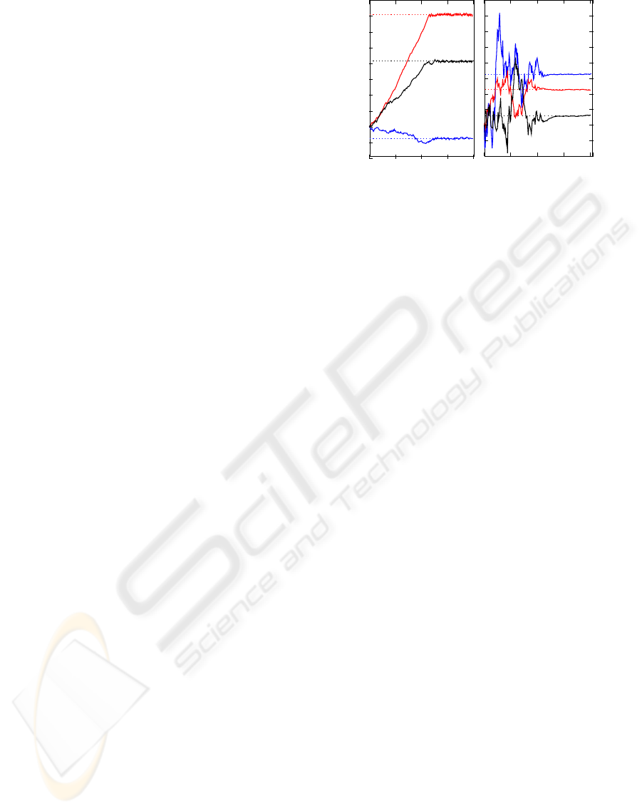
Figure 1: Convergence of the algorithm. The three vector
components are indicated by x, y and z. The dotted horizon-
tal lines are the true parameter values of rigid body trans-
formation and the solid lines show the evolution of the esti-
mated values using the learning algorithm.
of maximum variance in V . Putting (17) and (16) to-
gether shows that E decreases when moving from T
to T
†
. There is thus no local minima in E, so E is
a Lyapunov function of the system, which proves the
convergence.
6 EXPERIMENTS
The first experiment aims at illustrating the conver-
gence properties of the algorithm described above and
is performed in simulation. A rotation vector b
∗
and
a translation vector v
∗
were randomly generated. The
estimated rigid body transformation was initialized to
the identity b = v = 0 and the algorithm was run on
randomly generated points x
i
. The results can be seen
in Figure 1. One sees that both b and v converge to
b
∗
and v
∗
respectively, as is expected from the con-
vergence properties studied above.
The next experiment involves a tracking task in
a real stereo vision setting made of two low qual-
ity USB cameras mounted on a fixed support. Three
color patches were taped on the object to be tracked.
A software, based on the OpenCV library can track
color blobs and locate them in three dimensions. The
object was moved by hand, so the only information
about the position of the object is given by the stereo
vision system. So the real position of the object is
unknown, i.e., there is no ground truth.
Using the data recordedfrom the stereo vision sys-
tem, the position and orientation of the end-effector
were computed using two different algorithms, the it-
erative one described in this paper (5) and (6) and the
closed-form solution described in (Horn, 1987). This
algorithm finds the rigid body transformation by opti-
mizing a least square criterion similar to E(T) defined
VISAPP 2008 - International Conference on Computer Vision Theory and Applications
676

0 500 1000 1500 2000 2500 3000
50
52
54
56
58
60
62
Rotation angle (in degree)
0 500 1000 1500 2000 2500 3000
iterative solution closed-form solution
frames
frames
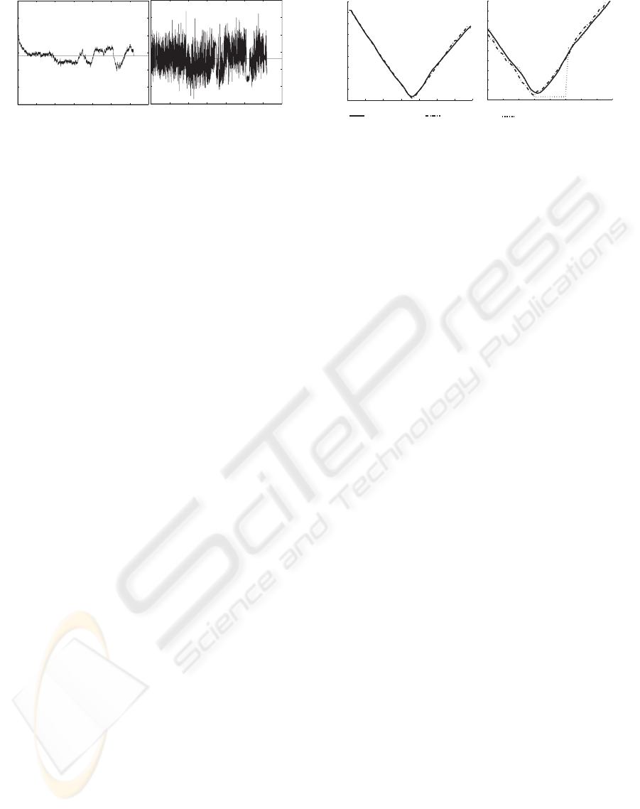
Figure 2: The behaviors of the tested algorithms in case of
noise in the data. The iterative algorithm (left graphs) is less
noisy than the closed-form algorithm. The object is static,
and the same data was used on both algorithms.
in (8).
In both cases, the data was taken as it is, without any
preprocessing. The iterative algorithm was initialized
using the closed-form algorithm on the initial patch
positions. In the absence of ground truth, the pre-
cision of the tracking algorithm is not investigated.
Rather, we compare the behaviors of the iterative and
closed-form algorithms
The first experiment was made with a static object.
Using the same marker position data coming from the
stereo vision software, we ran both algorithms to es-
timate the position and the orientation of the object.
The results can be seen in Figure 2. One sees that the
iterative solution is much less sensitive to noise in the
data. This is because the closed-form solution has no
memory, whereas the iterative solution can only up-
date its current estimate up to a certain amount, which
produces a smoothing effect.
The second experiment was made with a moving
object. In this experiment, the effect of missing points
is investigated. Two different scenarios were tested.
In the first scenario (periodic occlusion), a randomly
selected point was removed in each frame. In the sec-
ond scenario (lasting occlusion) a given point was re-
moved from the data for 10 consecutive frames. The
results can be seen in Figure 3. One sees that for both
scenarios, the closed-form algorithm (dotted lines)
cannot deal with the missing points as it requires at
least three concomitant points. To the contrary, the
iterative algorithm (dashed-dotted line) can deal with
the missing points as it has no such requirement. It
can follow pretty well the position given by the base-
line (solid line). This baseline was obtained by using
the closed-form algorithm and smoothing the result.
7 DISCUSSION
The results presented above show that an iterative so-
lution to a rigid body transformation can be advan-
0 10 20 30 40 50 60 70
0
10
20
30
40
50
60
70
80
90
frames
rotation angle (in degree)
20 25 30 35 40 45 50 55 60
0
5
10
15
20
25
30
35
40
45
50
frames
baseline
iterative solution
closed-form solution
periodic occlusion lasting occlusion
Figure 3: The behaviors of the tested algorithms in case
of occlusions. The iterative algorithm can deals well with
points periodically missing and points missing for a number
of consecutive frames (lasting occulsions).
tageous in a tracking application. The main advan-
tages come from the fact that the iterative solution
does not make the assumption that it has concomitant
points. Moreover, it ensures a continuity in the es-
timates, which is not guaranteed by the memoryless
closed-form solution. When using the iterative solu-
tion suggested here, the learning rate must be care-
fully chosen to be big enough to avoid loosing track
of the object, while remaining small enough to ensure
a smooth estimate of the transformation.
Although it was not investigated in this paper, we be-
lieve that the suggested algorithm could be useful in
other applications, especially in iterative algorithms
like ICP. This algorithm could also most probably be
easily extended to include uniform scaling of rigid
body transformations.
REFERENCES
Altmann, S. (1986). Rotations, Quaternions and Double
Groups, chapter 4, page 80. Oxford University Press.
Arun, K., Huang, T., and Blostein, S. (1987). Least-squares
fitting of two 3-d point sets. IEEE Transactions on
Pattern Analysis and Machine Intelligence.
Eggert, D., Lorusso, A., and Fisher, R. (1997). Estimating
3-d rigid body transformation: a comparison of four
major algorithms. Machine Vision and Applications.
Hestenes, D. (1999). New Foudations for Classical Me-
chanics, pages 277–305. Fundamental Theories of
Physics. Kluwer Academic Publishers, 2 edition.
Horn, B. (1987). Closed-form solution of absolute orien-
tation using unit quaternions. Journal of the Optical
Society of America A, 4(4):629–641.
Walker, M., Shao, L., and Volz, R. (1991). Estimating 3-
d location parameters using dual number quaternions.
CVGIP: Image Understanding.
ITERATIVE RIGID BODY TRANSFORMATION ESTIMATION FOR VISUAL 3-D OBJECT TRACKING
677