
EDGE-PRESERVING SMOOTHING OF NATURAL IMAGES BASED
ON GEODESIC TIME FUNCTIONS
Jacopo Grazzini and Pierre Soille
Spatial Data Infrastructures Unit
Institute for Environment and Sustainability
European Commission - DG Joint Research Centre
Via E.Fermi 2749, TP 262 - 21027 Ispra (VA), Italy
Keywords:
Mathematical morphology, edge-preserving smoothing, nonlinear filtering, geodesic time.
Abstract:
In this paper, we address the problem of edge-preserving smoothing of natural images. We introduce a novel
adaptive approach derived from mathematical morphology as a preprocessing stage in feature extraction and/or
image segmentation. Like other filtering methods, it assumes that the local neighbourhood of a pixel contains
the essential information required for the estimation of local image properties. It performs a weighted av-
eraging by combining both spatial and tonal information in a single similarity measure based on the local
calculation of geodesic time functions from the estimated pixel. By designing relevant geodesic masks, it
can deal with specific situation and type of images. We describe in the following two possible strategies and
we show their capabilities at smoothing heterogeneous areas while preserving relevant structures in natural -
greyscale or multispectral - images displaying different features.
1 INTRODUCTION
Image smoothing is a common preprocessing stage
used to improve the visual information in an image,
and to simplify subsequent image processing stages
such as feature extraction, image segmentation or mo-
tion estimation (J
¨
ahne, 1997). Traditionally, the prob-
lem of image smoothing is to reduce undesirable dis-
tortions - due to the presence of noise or the quality
of the image acquisition process - while preserving
important features such as homogeneous regions, dis-
continuities, edges and textures.
Smoothing techniques have been extensively used
in many fields of image processing (Saint-Marc and
Medioni, 1991; Winkler et al., 1999; Mr
´
azek et al.,
2006; Takeda et al., 2007). The generic continu-
ous expression of a low pass filtering (smoothing) of
an image f is the convolution operation of this im-
age (J
¨
ahne, 1997):
f (x)⊗K (x) =
Z
IR
2
K (x, y) f (y) dy (1)
where x = (x,y) are spatial coordinates, f (x) is the
local luminance (greylevel intensity or multispectral
value) in x and K is a kernel function (also called
”window function”) that is assumed to be normalised:
R
IR
2
K (x, y)dy = 1 and shift invariant: K (x, y) =
K (x −y). In practical case, the integral
R
IR
2
in Eq. (1)
becomes a discrete weighted summation
∑
ZZ
2
and the
support size of the kernel K is finite, as it is often
desirable to estimate the intensity of a pixel from a
local neighbourhood. Depending on the functional
form of the kernel, smoothing algorithms are classi-
fied into two categories: linear and nonlinear meth-
ods (J
¨
ahne, 1997), allowing for different weighting
of the luminance values. For linear smoothing, lo-
cal operators are uniformly applied to the image to
form the output luminance (van den Boomgaard and
van de Weijer, 2003). The most straightforward and
the fastest technique consists in using an isotropic ker-
nel, with fixed size and fixed weights, over the image.
Such approach yields good results when all the pix-
els in the window (i.e. the kernel support) come from
the same ’population’ as the central pixel: in image
regions corresponding to the interior of an object, it
produces a desirable luminance which is representa-
tive of the region. However, difficulties arise when
the window overlaps a discontinuity: on the bound-
aries between different regions, it results in averaging
of edge values, and therefore significant blurring of
the edges. Not only the noise is reduced but also the
image structures are smoothed. The problem remains
that a fixed kernel K is not suited for images featur-
20
Grazzini J. and Soille P. (2008).
EDGE-PRESERVING SMOOTHING OF NATURAL IMAGES BASED ON GEODESIC TIME FUNCTIONS.
In Proceedings of the Third Inter national Conference on Computer Vision Theory and Applications, pages 20-27
DOI: 10.5220/0001087400200027
Copyright
c
SciTePress

ing real structures on various scales and with differ-
ent shapes: there is a trade-off between localisation
accuracy and noise sensitivity. Nonlinear smoothing
has been developed to overcome these shortcomings,
which tend to preserve important features along with
noise removal during smoothing (Narendra, 1981;
Brownrigg, 1984; Perona and Malik, 1990; Nitzberg
and Shiota, 1992). In this context, the need for an
adaptive approach to cope with inhomogeneities in
images is well recognised (Saint-Marc and Medioni,
1991; Gomez, 2000; Grazzini et al., 2004). Strong
relations have been established between a number of
widely-used adaptive filters for digital image process-
ing (Mr
´
azek et al., 2006). The most common strategy
is to locally vary the kernel over image regions ac-
cording to their contents (Takeda et al., 2007): around
a pixel x to be updated, one uses a kernel K = K
x
with proper weights depending on the actual image
variability in the neighbourhood of x. A critical issue
is then how to measure image variability for gener-
ating the weights of the kernel. A possible approach
consists in adapting the local effect of the filter by
using both the location of the nearby samples and
their luminance values. That is, the proposed ker-
nel K
x
takes into account two factors: spatial dis-
tances |x −y| and tonal distances |f (x) − f (y)|. In-
troducing a tonal weight, the mixing of different lu-
minance ’populations’ is prevented. Such approach is
known as the bilateral filtering technique introduced
by (Tomasi and Manduchi, 1998) as an intuitive gen-
eralisation of the Gaussian convolution. In fact, it
is clear from the literature that there is a direct re-
lationship between this technique and other nonlinear
smoothing methods (van den Boomgaard and van de
Weijer, 2003; Mr
´
azek et al., 2006): anisotropic dif-
fusion (Barash, 2002), local-mode finding (van den
Boomgaard and van de Weijer, 2002) or mean-shift
analysis (Comaniciu and Meer, 2002).
Following the line of thought of (Tomasi and Man-
duchi, 1998), this paper introduces a new algorithm
for edge-preserving smoothing of natural images as a
preprocessing stage in feature extraction and/or image
classification. The present method exploits an image-
dependent approach derived from concepts known in
mathematical morphology (Soille, 2004). It is based
on the definition of appropriate geodesic masks and
the local estimation of pairwise geodesic time func-
tions within these masks (Lantu
´
ejoul and Maison-
neuve, 1984; Soille, 1994a; Soille, 1994b; Soille and
Grazzini, 2007). Likewise bilateral filtering, the main
idea is to associate with each pixel a weighted con-
volution of sample points within an adaptive neigh-
bourhood, where the weights depend not only on the
spatial distances but also on the tonal distance to the
centre pixel. With respect to other nonlinear tech-
niques, which often involve iterative operations (Per-
ona and Malik, 1990; Comaniciu and Meer, 2002),
this approach presents the advantage of not depending
upon any termination time. Moreover, it enables to
determine adaptively, directly from the unsmoothed
input data, the neighbouring sample points and the
associated weights. Namely, by designing relevant
geodesic masks, the geodesic time functions com-
puted from a single pixel provide a similarity measure
of the twofold spatial and tonal information in the lo-
cal neighbourhood of this pixel.
The rest of the paper is organised as follows. In
the next section, we recall the fundamental notions
of geodesic path, geodesic mask and geodesic time
known in mathematical morphology. In section 3, we
introduce a new filter for image smoothing based on
the estimation of local geodesic time on the gradient
magnitude. In section 4, we propose an alternative al-
gorithm based on the calculation of the geodesic time
on image variations able to deal with the presence of
noise. In section 5, we present and discuss some re-
sults and also compare the approach with other ex-
isting techniques. A conclusion regarding the current
results and a description of future foreseen develop-
ments are presented in section 6.
2 GEODESIC TIME ON
GREYLEVEL IMAGES
Geodesic transforms are classical operators in image
analysis (Lantu
´
ejoul and Maisonneuve, 1984; Verwer
et al., 1989). The geodesic distance between two pix-
els of a connected set (typically, a binary image) is de-
fined as the length of the shortest path(s) linking these
points and remaining in the set (the so-called geodesic
paths). This idea can been generalised to greylevel
images (images with single-valued luminance) using
the geodesic time on geodesic mask (Soille, 1994b;
Ikonen and Toivanen, 2007). In such case, the image
is then treated as a ’height map’, i.e. a surface embed-
ded in a 3D space, with the third coordinate given by
the greylevel values. The geodesic paths are then con-
strained to the surface of the height map: typically, the
path between two close pixels can be long, if there is
a high ’ridge’ in the greylevel map between them.
If we consider a greylevel image as an inte-
grable function g (designed as the geodesic mask), the
time τ
g
(P ) necessary for travelling on a path P de-
fined on the domain of definition of g is expressed as
the integral of g along P (Soille, 1994b):
τ
g
(P ) =
Z
P
|g(s)|ds . (2)
EDGE-PRESERVING SMOOTHING OF NATURAL IMAGES BASED ON GEODESIC TIME FUNCTIONS
21

The designation ’time’ is justified by considering
units equal to the inverse of that of a speed for the
image g. Following, the geodesic time τ
g
(p,q) sep-
arating two points p and q is the smallest amount of
time allowing to link p to q in g:
τ
g
(p,q) = min{τ
g
(P ) | P is a path linking p to q}.
In the discrete case, a path P of length l going from p
to q is defined as a l-tuple (x
1
,...,x
l
) of pixels such
that x
1
= p, x
l
= q, and (x
i−1
,x
i
) defines adjacent pix-
els for all i ∈ [2,l]. Therefore, the greylevel values
intuitively represent the cost of traversing the pixels:
the lower the greylevel value, the faster the propaga-
tion. More precisely, the cost c
i
of travelling from a
pixel x
i
to an adjacent pixel x
i+1
is
1
:
c
i
=
1
2
(g(x
i
) + g(x
i+1
)) ·|x
i
−x
i+1
| (3)
where the spatial distance |x
i
−x
i+1
| can be either the
Euclidean distance or the optimal Chamfer propagat-
ing weights in a binary 3×3 mask (Borgefors, 1986).
The time τ
g
(P ) necessary to cover a discrete path P
then refers to the sum of the greylevel values of the
pixels along P ; the geodesic time τ
g
(p,q) finds the
path with the lowest sum of greylevel values along all
possible discrete paths linking p to q. This concept is
closely related to the notion of grey weighted distance
transform defined in (Levi and Montanari, 1970) and
to the continuous formulation of the eikonal equa-
tion (Cohen and Kimmel, 1997).
3 SMOOTHING FILTER
DERIVED FROM LOCAL
GEODESIC TIME ON
GRADIENT MAGNITUDE
In many adaptive smoothing techniques, a way to cir-
cumvent mixing the values from different populations
is to introduce a similarity measure between the pix-
els of the image. We observe in particular that calcu-
lating the tonal weight in bilateral filtering (Tomasi
and Manduchi, 1998) implicitly introduces an esti-
mate of the local gradient between neighbouring val-
ues, then using this estimate to weight the respective
measurements. Accordingly, we propose to combine
both spatial and tonal information into a single simi-
larity measure by estimating locally the geodesic time
1
A reason why we do not use the term ’distance’ for de-
signing this geodesic function is precisely Eq. (3): indeed,
it appears possible for the cost c
i
to be null between two
adjacent pixels.
with the magnitude of the spatial gradient of the im-
age as the geodesic mask. A related concept was de-
scribed in (Sumengen et al., 2006) within the continu-
ous framework of the eikonal equation for image seg-
mentation. The underlying idea is that the geodesic
paths associated to this function define the intrin-
sic neighbourhood relationship between the sample
points when the 2D image is projected onto the 3D
spatial-tonal domain (the ’height map’ described ear-
lier).
The values of the magnitude of the spatial gra-
dient |∇ f | of the image f are regarded as the cost
of crossing a pixel. By replacing the function g
by |∇ f | in Eq. (3), it implies that the time neces-
sary to travel between two pixels separated by high
gradient values is higher than the time necessary to
travel between two pixels separated by low gradient
values. In the case of multivalued image, the cal-
culation of the geodesic time must however be con-
sidered carefully, either processing channel by chan-
nel (i.e. calculating local gradient and local geodesic
time separately for each band), or processing si-
multaneously the information provided by the dif-
ferent channels of the image (i.e. using an estima-
tion of the local multispectral gradient). The ma-
jor advantage of the second approach is that it is
taking into account the actual multispectral edge in-
formation, so further smoothing will be more effi-
cient along edges, and, thus, edges will be better pre-
served. A way to estimate the gradient magnitude
of a multichannel image f with components f
n
,n =
1,...,N is by means of the eigenvalue analysis of
the image squared differential proposed in (Di Zenzo,
1986), expressed by the so-called 2 ×2 matrix called
first fundamental form (Scheunders and Sijbers,
2001):
h
∑
n
(
∂ f
n
∂x
)
2
,
∂ f
n
∂x
∂ f
n
∂y
;
∑
n
∂ f
n
∂x
∂ f
n
∂y
,
∑
n
(
∂ f
n
∂y
)
2
i
. The
direction of maximal and minimal change are given
by the eigenvectors of this matrix while the corre-
sponding (positive) eigenvalues λ
1
≥ λ
2
denote the
rate of change. In particular, for greylevel images
(N = 1), it is verified (Scheunders and Sijbers, 2001)
that the largest eigenvalue is given by the squared
gradient magnitude: λ
1
= |∇ f |
2
and the correspond-
ing eigenvector lies in the direction of the gradient.
Therefore, taking into account these observations, we
select the locally defined function λ
1
(or indifferently
√
λ
1
) as the natural estimate for the gradient magni-
tude of the image
2
.
For each pixel x, the similarity measure to all
other pixels in its neighbourhood can then be com-
2
λ
1
is naturally used as being the derivative energy in the
most prominent direction, but other measure can be consid-
ered, e.g., λ
1
−λ
2
which is similar to λ
1
corrected for the
energy contributed by noise (Sapiro and Ringach, 1996).
VISAPP 2008 - International Conference on Computer Vision Theory and Applications
22

puted as a (monotonically) decreasing function K of
the geodesic time τ
g
(x,·) from x within the geodesic
mask g(x) = λ
1
(x). Classically, a Gaussian func-
tion G
σ
with standard deviation σ will provide desir-
able results:
K (x, y) = G
σ
(τ
g
(x,y)) = exp {
R
y
x
λ
1
(s)ds
σ
2
} (4)
but other kernels are not excluded. We can finally
perform a weighted average of local samples by ap-
plying Eq. (1) with this kernel (figure 1, top). This
way, the effective sampling procedure of the pixels y
used for estimating the value of the central pixel x
is adapted locally to image features such as edges.
Indeed, larger weight should be assigned to pixels y
that involve low gradient values along the minimal
geodesic paths from x, and vice versa. In particu-
lar, luminance values from across a sharp feature are
given less weight because they are penalised by the
time on the gradient magnitude. In practise, due to
memory and computational limitations, the support
of K is limited to a fixed size, i.e. sample pixels y that
are further away (in the spatial domain) than a fixed
distance ω (e.g. given by an analysing window Ω)
to the central pixel x are not considered. Moreover,
we introduce a parameter α which controls the global
strength of the smoothing: the geodesic mask is re-
fined and replaced by g(x) = α ·λ
1
(x). When α in-
creases, the geodesic time on the embedded surface
becomes more sensitive to image deformations: the
cost of crossing a pixel increases. α controls the rela-
tive influences of tone and space in the calculation of
the similarity measure of neighbour pixels.
Algorithms based on priority queue data struc-
tures (Soille, 1994b), implementing Dijkstra algo-
rithm, enable an efficient implementation of the lo-
cal geodesic time with a computational complexity of
O(ω
2
logω
2
) (Ikonen, 2007). They take advantage of
the fact that the analysing windows Ω are finite and
totally ordered, and they guarantee that pixels that ef-
fectively contribute to the output are processed only
once. Thus, running the algorithm calculating the lo-
cal geodesic time from each pixel in the image results
in a total complexity of O(w ·h ·ω
2
logω
2
) where w
and h are respectively the width and the height of the
input image.
4 DENOISING FILTER DERIVED
FROM LOCAL GEODESIC
TIME ON IMAGE VARIATIONS
It is well-known that discontinuities in an image likely
correspond to important features. However, noise cor-
ruption can generate discontinuities as well. There-
fore, how to measure significant discontinuities is a
nontrivial problem. In particular, spatial gradient is
known to be quite sensitive to noise. Owing to over-
locality, it is inadequate to detect significant discon-
tinuities from a noisy image, which usually causes
adaptive smoothing algorithm based on gradient in-
formation to yield poor results. To tackle this prob-
lem, measures of higher order differentiations have
been proposed (Nitzberg and Shiota, 1992). How-
ever, these techniques involve higher computational
complexity since usually, in those approaches, a dis-
continuity measure has to be used in each iteration of
adaptive smoothing.
In order to have both a strong denoising effect and
a sharper image, we define a geodesic time that ac-
counts for both the distance between pixels and the
roughness of the ’height map’, i.e. a measure of the
shortest path drawn on the projection of the 2D image
onto the spatial-tonal domain. For this purpose, we
express the geodesic time in the continuous case by:
τ
g
(P ) =
Z
P
|
dg(s)
ds
|ds . (5)
so that the cost c
i
of crossing pixels becomes:
c
i
=
1
2
|g(x
i
) −g(x
i+1
)|·|x
i
−x
i+1
| (6)
with the distance |x
i
−x
i+1
| defined as before. The
similarity measure is then estimated by setting the
geodesic mask to the input noisy image: g(x) = f .
This definition derives from the so-called weighted
distance on curves space of (Ikonen and Toivanen,
2007), where the multiplication in Eq. (6) is replaced
by an addition. Its intuitive interpretation is that it rep-
resents the minimal amount of ascents and descents
to be travelled to reach a neighbouring pixel. This
notion also expresses a similar geometric notion as
the path variation defined in (Arbel
´
aez and Cohen,
2003). Note that in fact the geodesic mask associ-
ated to the time τ
g
(P ) of Eq. (5) is constantly updated
through the propagation of the geodesic time (Ikonen
and Toivanen, 2007; Ikonen, 2007). For multichan-
nel images f , the norm in Eq. (6) must be under-
stood as a multispectral norm, e.g the L
∞
norm on
the different channels; in such case, we have, when
estimating the minimal path, |g(x
i
) −g(x
i+1
)| ≤ t if
and only if |f
n
(x
i
)− f
n
(x
i+1
)|≤t for all n = 1,..., N.
As a consequence, this approach depends, like bilat-
eral filtering (figure 1, bottom right) and contrary to
the one presented in the previous section, on the di-
mension of the tonal space. Whereas the formulation
with Eq. (2) was going through the lowest values of
the spatial gradient (the mask being defined as a func-
tion g(x) ∼ |∇(x)|), the geodesic time defined with
EDGE-PRESERVING SMOOTHING OF NATURAL IMAGES BASED ON GEODESIC TIME FUNCTIONS
23
Eq. (5) (and g(x) ∼ f (x)) minimises the changes in lu-
minance values. Image denoising is finally performed
using a kernel like Eq. (4), and introducing similarly a
multiplicative control parameter α on the smoothing
(figure 1, bottom left).
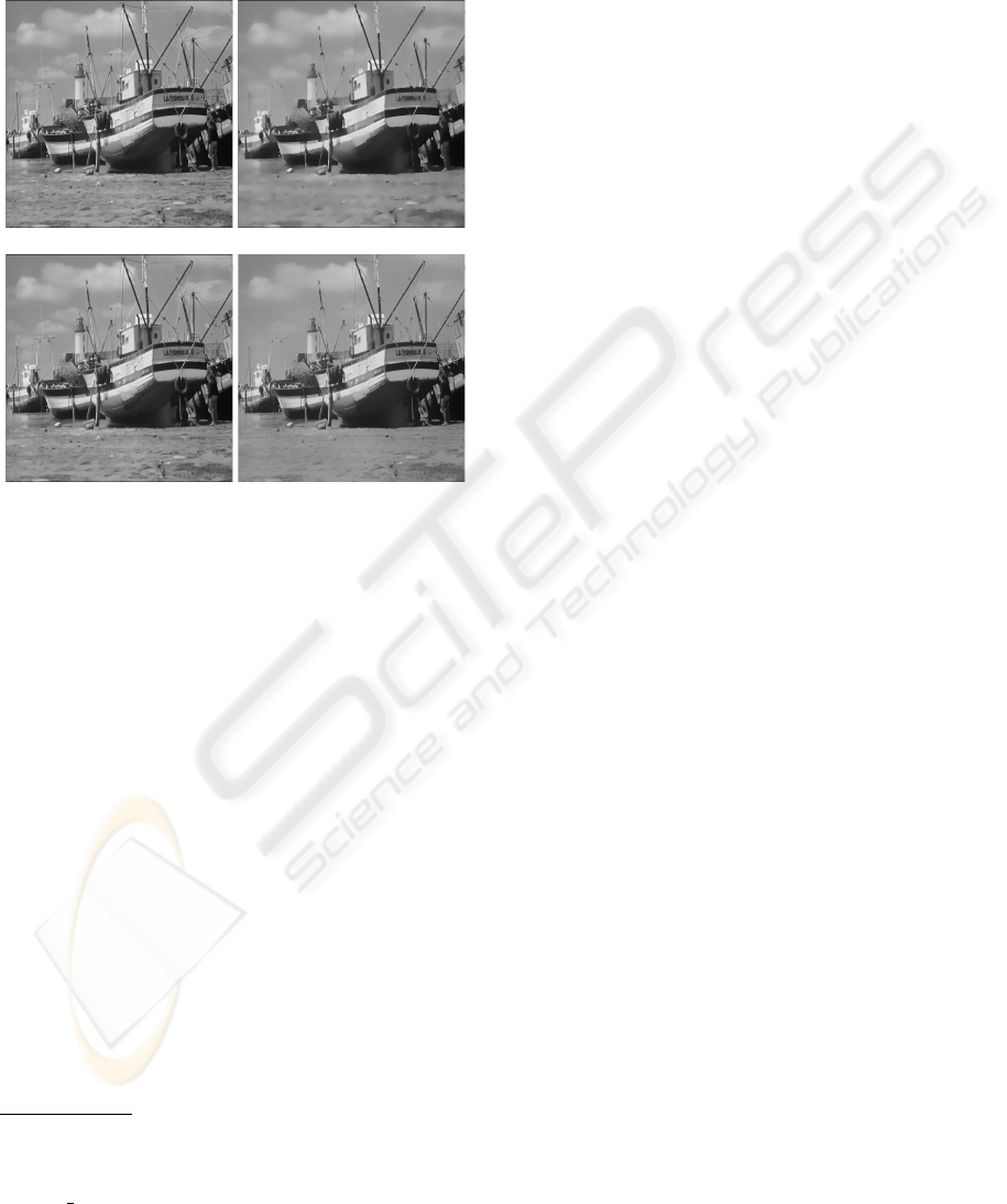
Figure 1: Results of smoothing applied on the image of the
boat La Cornouaille. Top: smoothing using the filter based
on the magnitude of the gradient as described in section 3
with a control parameter α = 20 (left, soft smoothing effect)
and α = 5 (right, strong smoothing). Bottom: smoothing
using the filter described in section 4 based on the image
variations with α = 20 (left) and the output of some bilateral
filtering (right). For both ’geodesic’ filters, the parameters
σ = 1 and ω = 21 were fixed.
5 EXPERIMENTS AND
COMPARISON WITH OTHER
TECHNIQUES
We show in this section the results of the new pro-
posed algorithms applied on different types of im-
ages
3
: greylevel or multispectral, displaying different
typical features: texture, edges or noise. Depending
on the input data and the final purpose, we choose to
employ one of the two approaches: smoothing and
image simplification with the algorithm described in
section 3, denoising with the algorithm of section 4.
3
Consult the online USC database http://sipi.usc.
edu/database/database.cgi?volume=misc and the web-
page http://homepages.inf.ed.ac.uk/rbf/CVonline/
LOCAL COPIES/GOMEZ1/results.html of (Gomez,
2000) for the original sample images.
Both filtering techniques result in visually satis-
fying smoothed versions of the original images (fig-
ure 1). Indeed, the generic approach enables to
conserve features through the combined spatial and
tonal actions represented in the similarity measure
based on the geodesic time functions. Both filters
nicely smooth homogeneous areas while preserving
important structures such as the boundaries of ob-
jects. Close inspection to the images also shows they
are good at enhancing subtle texture regions and they
suppress small elements corresponding to the main
heterogeneity (figure 2). The image structures are
not geometrically damaged, what might be fatal for
further processing like classification or segmentation.
Indeed, it creates homogeneous regions instead of
points or pixels as carriers of features which should be
introduced in further processing stages. The amount
of smoothing can be controlled by the parameter α
(figure 2(a)). With a small α value, the estimated
image will be much smoother so that details have
been sacrificed to the effect of denoising, producing
a gaussian-like blurring effect. High values of α pre-
serve almost all contrasts, and thus lead to filters with
little effect on the image. For intermediate values of
α, the filtering procedures result in a diffusion ef-
fect, amplifying or attenuating the given local con-
trast in parts of an image. The filter based on gra-
dient’s magnitude show higher capability at blurring
small discontinuities and sharpening edges when ap-
plied on noise-free images (figure 2(b)), whereas the
filter based on image variations performs better when
dealing with noisy images (figure 3). The intrinsic
dependence of the latter filter on the luminance dif-
ferences allows one to give less influence to outlier
pixels when denoising (suppressing peaks in lumi-
nance distribution). A possible improvement when
smoothing an image also regards the input central
pixel value f (x). As underlined in (van den Boom-
gaard and van de Weijer, 2002), using this value as
the ’reference’ for the estimation of the local geodesic
time assumes that it is more or less noise free. This
is naturally a questionable assumption when building
a noise suppression filter and may have effect on the
result. Following the authors’ suggestion we could re-
place the central pixel’s value with some estimate of
the true value, e.g. the median value in an window of
size 3 ×3.
As discussed in the introduction (section 1), the
bilateral filter of (Tomasi and Manduchi, 1998) uses,
as a simple and intuitive choice of the adaptive ker-
nel, separate terms for penalising the spatial and tonal
distances. In practise, Gaussian influence weight-
ing functions are used. Our filters and the bilat-
eral one result in very similar smoothed images (fig-
VISAPP 2008 - International Conference on Computer Vision Theory and Applications
24
(a) Influence of the control parameter α on the ’geodesic’
filters, resp. based on the gradient’s magnitude (first row,
with α = 1 and α = 20), and on image variations (second row,
with α = 5 and α = 10); the parameters σ = 1 and ω = 11 were
fixed.
(b) Outputs of smoothing performed on a detail of the man-
drill (top left) with some bilateral filter (top right) and the
filters based resp. on the gradient’s magnitude (bottom left)
and image variations (bottom right); the parameters for both
’geodesic’ filters are α = 10, ω = 11 and σ = 1.
Figure 2: Smoothing applied to the mandrill image.
ure 2(b)). However, breaking the filtering kernel into
spatial and tonal terms weakens the estimator perfor-
mance since it limits the degrees of freedom and ig-
nores correlations between the positions of the pixels
and their values. Using a twofold similarity measure
like the geodesic time, defined on either the spatial
gradient or the image variation, enables to account
for these correlations. A smoothing technique de-
scribed in (Gomez, 2000) is based on adaptive Gaus-
sian filters. It adjusts locally the smoothing scale
(i.e. the standard deviation of the Gaussian kernel)
in a scale-space framework, through a minimal de-
scription length criterion. This way, the resulting
smoothed data values intuitively share, at every loca-
tion, a similar signal-to-noise ratio. Likewise the ap-
proach described in section 4, it is not based on partial
derivatives. However, this approach results in blurred
images when used for denoising (figure 3). Compared
to iterative schemes like anisotropic diffusion (Perona
and Malik, 1990), our approach is a non-iterative es-
timation technique, which makes it more efficient and
more stable (figure 3).
6 CONCLUSIONS
In this paper, we explore the use of geodesic time
functions for edge-preserving smoothing of natural
images. The basic idea is similar to that of spatial-
tonal filtering approaches, which consist in employ-
ing both geometric and luminance closeness of neigh-
bouring pixels. The originality of the approach we
propose lies in the definition of a new similarity mea-
sure combining both spatial and tonal information
and based on the local estimation of some geodesic
time functions. We show that, by designing relevant
geodesic masks, we can define new smoothing filters
enable at simplifying and/or denoising images, de-
pending on the input data and on the target purpose.
Finally, the proposed techniques show good results in
different situations and images, where they were able
to preserve the main structures, such as edges and
textures, while smoothing other homogeneous parts.
Likewise other spatial-tonal based techniques, the de-
gree of smoothing in the image can also be controlled
in order to adjust the fidelity to the original image.
Current research is geared towards improving and
extending the present work. Improvements regard
mainly the parameters’ selection. There is in particu-
lar an issue regarding the spatial extent of the window
used for estimating the local geodesic time functions.
In this paper, we used a finite spatial window Ω with
size ω for limiting the calculations. An alternative
approach would be to limit the weighting average to
the sample pixels reached from the central pixel with
a time inferior to a given threshold value. This way,
it would be possible to determine when the neighbour
EDGE-PRESERVING SMOOTHING OF NATURAL IMAGES BASED ON GEODESIC TIME FUNCTIONS
25
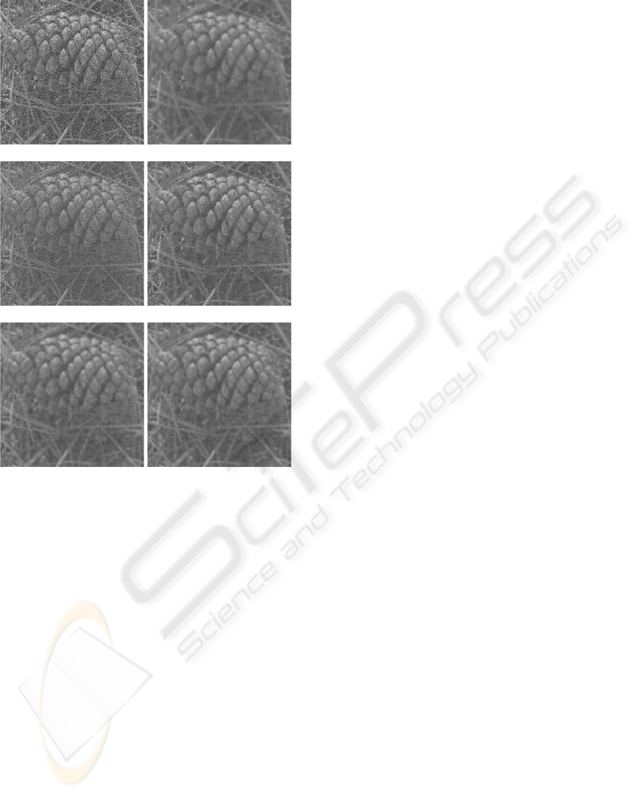
Figure 3: The results of smoothing of the pine cone im-
age corrupted with Gaussian noise (detail, top left) are dis-
played, in this order, for: the method of (Gomez, 2000),
some bilateral filter according to (Tomasi and Manduchi,
1998), anisotropic diffusion following (Perona and Malik,
1990) and the ’geodesic’ filters based on gradient magni-
tude and image variations.
pixels must be considered as outliers. The selection of
the smoothing control parameter α should also be in-
vestigated. Another issue regards directly the estima-
tion of the local geodesic time: the calculation could
be refined by normalising locally the local cost of
pixel crossing, i.e. considering c
i
/max {c
i
| x
i
∈ Ω}
in the geodesic propagation instead of c
i
currently. A
natural extension to our approach is to consider me-
dian filtering instead of weighted averaging of the pix-
els in local neighbourhoods. Selecting the (weighted)
median rather than the mean helps to prevent outlier
pixels from unduly distorting the result.
We believe that the proposed techniques are of
particular interest for filtering data for which a dis-
crete approach should be adopted, instead of a contin-
uous one, in order to avoid creating spurious artifacts
through diffusion-like processes. We foresee in par-
ticular potential applications in the fields of medical
imaging and remote sensing.
REFERENCES
Arbel
´
aez, P. and Cohen, L. (2003). Path variation and image
segmentation. In Proc. of EMMCVPR, volume 2683
of LNCS, pages 246–260. Springer.
Barash, D. (2002). A fundamental relationship between bi-
lateral filtering, adaptive smoothing and the nonlinear
diffusion equation. IEEE Trans. Patt. Ana. Mach. In-
tel., 24(6):844–847.
Borgefors, G. (1986). Distance transformations in digital
images. Comp. Vis. Graph. Im. Proc., 34:344–371.
Brownrigg, D. (1984). The weighted median filter. Comm.
of ACM, 27(8):807–818.
Cohen, L. and Kimmel, R. (1997). Global minimum for
active contour models: a minimal path approach. Int.
J. Comp. Vis., 24:57–78.
Comaniciu, D. and Meer, P. (2002). Mean shift: a robust
approach toward feature space analysis. IEEE Trans.
Patt. Ana. Mach. Intel., 24(5):603–619.
Di Zenzo, S. (1986). A note on the gradient of a multi-
image. Comp. Vis. Graph. Im. Proc., 33:116–125.
Gomez, G. (2000). Local smoothness in terms of variance.
In Proc. of BMVC, volume 2, pages 815–824.
Grazzini, J., Turiel, A., Yahia, H., and Herlin, I. (2004).
Edge-preserving smoothing of high-resolution images
with a partial multifractal reconstruction scheme. In
Proc. of ISPRS, pages 1125–1129.
Ikonen, L. (2007). Priority pixel queue algorithm for
geodesic distance transforms. Im. Vis. Comp.,
25:1520–1529.
Ikonen, L. and Toivanen, P. (2007). Distance and near-
est neighbor transforms on gray-level surfaces. Patt.
Recogn. Lett., 28:604–612.
J
¨
ahne, B. (1997). Digital Image Processing: Concepts, Al-
gorithms and Scientific Applications. Springer-Verlag.
4
th
edition.
Lantu
´
ejoul, C. and Maisonneuve, F. (1984). Geodesic meth-
ods in image analysis. Patt. Recogn., 17:177–187.
Levi, G. and Montanari, U. (1970). A grey-weighted skele-
ton. Inform. Cont., 17:62–91.
Mr
´
azek, P., J. Weickert, J., and Bruhn, A. (2006). On robust
estimation and smoothing with spatial and tonal ker-
nels. In Klette, R., Kozera, R., Noakes, L., and Weick-
ert, J., editors, Geometric Properties from Incomplete
Data, pages 335–352. Springer.
Narendra, P. (1981). A separable median filter for image
noise smoothing. IEEE Trans. Patt. Ana. Mach. Intel.,
3(1):20–29.
Nitzberg, M. and Shiota, T. (1992). Nonlinear image filter-
ing with edge and corner enhancement. IEEE Trans.
Patt. Ana. Mach. Intel., 14(8):826–833.
VISAPP 2008 - International Conference on Computer Vision Theory and Applications
26

Perona, P. and Malik, J. (1990). Scale space and edge de-
tection using anisotropic diffusion. IEEE Trans. Patt.
Ana. Mach. Intel., 12:629–639.
Saint-Marc, P. Chen, J. and Medioni, G. (1991). Adap-
tive smoothing: A general tool for early vision. IEEE
Trans. Patt. Ana. Mach. Intel., 13:514–529.
Sapiro, G. and Ringach, D. (1996). Anisotropic diffusion
of multivalued images with applications to color fil-
tering. IEEE Trans. Im. Proc., 5(11):15–82.
Scheunders, P. and Sijbers, J. (2001). Multiscale anisotropic
filtering of color images. In Proc. of IEEE ICIP, vol-
ume 3, pages 170–173.
Soille, P. (1994a). Generalized geodesic distances applied
to interpolation and shape description. In Serra, J.
and Soille, P., editors, Mathematical Morphology and
its Applications to Image Processing, pages 193–200.
Kluwer Academic Publishers.
Soille, P. (1994b). Generalized geodesy via geodesic time.
Patt. Recogn. Lett., 15(12):1235–1240.
Soille, P. (2004). Morphological Image Analysis: Princi-
ples and Applications. Springer-Verlag.
Soille, P. and Grazzini, J. (2007). Extraction of river net-
works from satellite images by combining mathemati-
cal morphology and hydrology. In Proc. of CAIP, vol-
ume 4673 of LNCS, pages 636–644. Springer-Verlag.
Sumengen, B., Bertelli, L., and Manjunath, B. (2006). Fast
and adaptive pairwise similarities for graph cuts-based
image segmentation. In Proc. of IEEE POCV.
Takeda, H., Farsiu, S., and Milanfar, P. (2007). Kernel
regression for image processing and reconstruction.
IEEE Trans. Im. Proc., 16(2):349–366.
Tomasi, C. and Manduchi, R. (1998). Bilateral filtering for
gray and color images. In Proc. of ICCV, pages 839–
846.
van den Boomgaard, R. and van de Weijer, J. (2002). On the
equivalence of local-mode finding, robust estimation
and mean-shift analysis as used in early vision tasks.
In Proc. of ICPR, volume 3, pages 927–930.
van den Boomgaard, R. and van de Weijer, J. (2003). Lin-
ear and robust estimation of local image structure. In
Proc. of Scale-Space, volume 2695 of LNCS, pages
237–254. Springer.
Verwer, B., Verbeek, P., and Dekker, S. (1989). An efficient
uniform cost algorithm applied to distance transforms.
IEEE Trans. Patt. Ana. Mach. Intel., 11(4):425–429.
Winkler, G., Aurich, V., Hahn, K., and Martin, A.
(1999). Noise reduction in images: some recent edge-
preserving methods. Patt. Recogn. Im. Ana., 9(4):749–
766.
EDGE-PRESERVING SMOOTHING OF NATURAL IMAGES BASED ON GEODESIC TIME FUNCTIONS
27
