ANOMALY DETECTION WITH LOW-LEVEL PROCESSES IN
VIDEOS
Ákos Utasi and László Czúni
Department of Image Processing and Neurocomputing, University of Pannonia, Egyetem str., Veszprém, Hungary
Keywords: Anomaly detection, motion vector, Mixture of Gaussian Modelling (MOG), probability estimation.
Abstract: In our paper we deal with the problem of low-level motion modelling and unusual event detection in urban
surveillance videos. We model the direction of optical flow vectors at image pixels. We implemented and
tested probability based approaches such as probability estimation, Mixture of Gaussians modelling, and
spatial averaging (with Mean-shift segmentation). We propose a Markovian prior to get reliable spatio-
temporal support. We tested the techniques on synthetic and real video sequences.
1 INTRODUCTION
We investigate the use of some low-level techniques
for the analysis of dense optical flow directions
without object level understanding. Since often the
frame rate of surveillance videos is not stable we
don’t consider the magnitude of motion vectors. In
our discussion we call a motion event unusual at any
location if the observed direction is implausible
assuming an unsupervised training phase with
normal observations. A good survey of visual
surveillance can be found in (Weiming, 2004). As
discussed in several papers (Dick, 2003; Pavlidis
2001) surveillance applications face a lot of
problems: optical distortion; electronic noise;
vibration/shaking of the camera; flicker; spatial or
temporal aliasing errors; compression artefacts;
weather conditions; head light glare; occlusion; non-
rigid motion; shadows; etc. Due to the limited size
of this paper we just mention some of the interesting
approaches. (Boiman, 2005) uses space-time video
segments measured relative to all the other video
segments. In (Andrade, 2005; Nair, 2002) the
anomalies of optical flow are analyzed with the help
of HMMs (Hidden Markov Models) while (Brand,
2000) uses a modified version of HMMs.
2 PREPROCESSING
We apply a Mixture of Gaussians (MOG) change
detection algorithm to exclude non-changing areas
from further analysis (Stauffer, 1999). For optical
flow calculation we used the multi-scale gradient
method of Bergen (Bergen, 1990). To filter the
optical flow vectors we applied several steps: only
pixels of the foreground mask were considered with
magnitude within a given range. To minimize the
number of unreliable motion vectors at large
homogenous areas we used vectors only around edge
pixels (detected with the Previtt operator followed
by two steps of dilation). We assumed that the
motion of objects is almost linear in a relatively
short period so we neglected those vectors which
showed larger deviation than 10 degrees from one
frame to the other.
3 DIRECTION MODELLING
3.1 Estimation of Probabilities
We collected 8-bin motion direction histograms for
all image pixels. Larger number of bins could
enhance the adaptation ability but would also
increase the uncertainty (since the learning time is
limited and there is no guarantee to get a continuous
distribution during learning). We supposed that the
relative occurrence of motion vectors gives a simple
but effective estimate of the empirical probability:
∑
=
Dir
DirDirDir
OOP
where
Dir
O
is the number of
observations in one of the predefined direction
classes
},,,,,,,{ NWSWSENEWSENDir
∈
.
678
Utasi Á. and Czúni L. (2008).
ANOMALY DETECTION WITH LOW-LEVEL PROCESSES IN VIDEOS.
In Proceedings of the Third International Conference on Computer Vision Theory and Applications, pages 678-681
DOI: 10.5220/0001087806780681
Copyright
c
 SciTePress

The probability that an observed vector belongs to
an unusually moving object is
Dir
Dir
U
PP −= 1
)(
.
Please note, that in the other two methods we used
the same approach but there Dir can take a
continuous value (Section 3.2 and 3.3).
3.2 Mixture of Gaussians (MOG)
If the number of samples during training is limited
then a set of Gaussian functions can be aligned to
the sparse data set. In (Stauffer, 1999) an adaptive
algorithm is proposed to update the parameters of
the MOG model used for motion detection. While in
case of background modelling the background pixels
change their values roughly periodically, in the
current case we observe recurrence in longer periods
so there is a doubt that the method of (Stauffer,
1999) can be applied successfully after a random
initialization of distributions. Consider K Gaussian
distributions with the probability density function:
∑
=
Σ=
K
i
titittit
xNxP
1
,,,
),|()( μω
, where
ti ,
ω
is the
weight,
ti,
μ
is the expected value, and
ti,
Σ is the
covariance of Gaussian distributions (N). The
algorithm has to decide if a new observation
t
x is
matching with any Gaussians in the mixture.
According to (Stauffer, 1999) if an observation is
within 2.5
σ
from the expected value of a
distribution then we consider the observation
matching the distribution. Denote the set of weights
of the matching distributions
with
{
}
;,
21 k
mmm
wwwW …= Km
i
≤≤1 . Then
the probability that the observation is usual:
}max{WP =
and
}{maxarg
max
Wm
i
m
=
. In each
step (frame) we update the weights for all
distributions as
(
)
ti
M
ti
ti ,
1,
1
,
αωαω +
−
−= and
the expected value
()()
dusigndsignd
tt
××+=
−
)(
1801
ρμμ
and
variance
2
180
2
1
2
')1( d
tt
ρσρσ +−=
−
for the matching
distribution. We
denote
tmt ,
max
μ
μ
=
,
2
,
2
max
tmt
σσ =
1−
−=
tt
xd
μ
,
tt
xd
μ
−=
′
||180180
180
dd −−=
,
dd
′
−−=
′
180180
180
1)180(2)(
0
−
−
= zHzu
(
0
H
is the Heaviside function), and
α
is the
learning factor. M equals 1 if the distribution
matches the current direction, otherwise M is 0, and
(
)
ttt
xN
Σ
=
,|
μ
α
ρ
. It is common to give
ρ
a
constant value, in our case
ρ
is set to 0.15. After
each update the weights are normalized.
3.3 Means-shift (MS) Segmentation
We investigated the Mean Shift segmentation
(Bogdan, 2003) of the probabilities as an extension
of the method of Section 3.1. We set the minimum
area of image segments typically between 200 and
4000 pixels (for close and distant recordings
respectively). The weights (“bandwidth”) of spatial
(x, y) coordinates is 7 while for the other dimensions
(the 8 direction bins) we set it 3 as proposed in
(Bogdan, 2003). The centre of Figure 1 illustrates
the estimated and the segmented motion statistics
(using a discriminating colouring algorithm). In the
event detection phase, we used the segmented
probability map for the estimation of anomalous
motion:
Dir
PiDir
SP = where },....,{
21 Ni
SSSSS =
∈
and
],,,...,[
00 Dirnni
PyxyxS
=
. Each segment
i
S is a
connected component of the image labelled with a
probability distribution
Dir
P obtained by
segmentation.
3.4 Markovian Extension
We can assume that unusual events happen at least
on two consecutive frames supposing a Markov
Chain property of objects’ motion. Thus if we found
an anomalously moving pixel and we estimated its
motion direction at time t then projecting back (with
motion compensation) to the preceding frame there
should also be a corresponding anomalous pixel with
high probability. This is formalized as:
}{max
1,',',
)(
','
,,,
)(
,,
),(
−
∈
⋅=
tyxDir
U
Ryx
tyxDir
U
tyx
MU
PPP
where
the second term of the product means that we use the
highest probability value of unusual observations
(
Dir
U
P
)(
) in the R neighbourhood (a box of size
5x5) of the motion compensated position (x’,y’).
4 EXPERIMENTS
We analyzed videos of different sceneries, types of
traffic, resolution, and quality
(http://www.knt.vein.hu/~czuni/visapp). For training
ANOMALY DETECTION WITH LOW-LEVEL PROCESSES IN VIDEOS
679

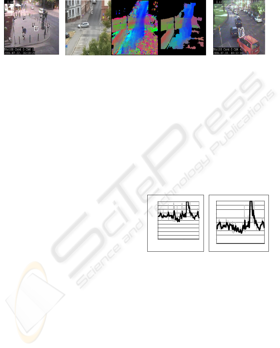
Figure 1. Anomalous objects are detected (with the method of Section 3.1) and marked with white outline. In the centre we
show raw and segmented direction probabilities, rendered with different colours.
we used 2000-10000 frames depending on the frame
rate and intensity of traffic. In the synthetic video
(“Syn”, @320x240, 25fps) we inserted several
textured rectangles moving to the left and to the
right with various speeds over a static background.
The sequence was loaded with Gaussian noise of
deviation 10 and we inserted a block moving up as
an anomalous object. The “Crossing” sequence
(@320x366, 8fps) shows a one-way street where
cars and pedestrians cross the street, a tree is waving
occasionally and shadows appear according to
weather. The selected frame shows a detected small
sized bicycle coming down in the wrong direction.
The third sequence (“Lanes”, @320x240, 5-15fps)
shows a busy road. We expect the algorithm to find
some pedestrians crossing the road horizontally and
some lane crossings are also anomalous.
5 EVALUATIONS
We can monitor the probability of events
continuously by
Dir
U
P
)(
and
Dir
MU
P
),(
defined by
one of the three described models. While basically
we apply pixel based processing we can still group
the local estimates with a simple method: we
labelled all connected components (above the size of
10-30 pixels) of the binary foreground image with
the average probability. We plot the probability of
the most suspicious blob (with the highest value).
Due to the limited space a few are selected for
presentation (for more see http://www.knt.vein.hu/
~czuni/visapp). The graphs show the probability as a
function of frame number. The dark trend line is the
smoothed version of the grey considered as the final
output of the detector.
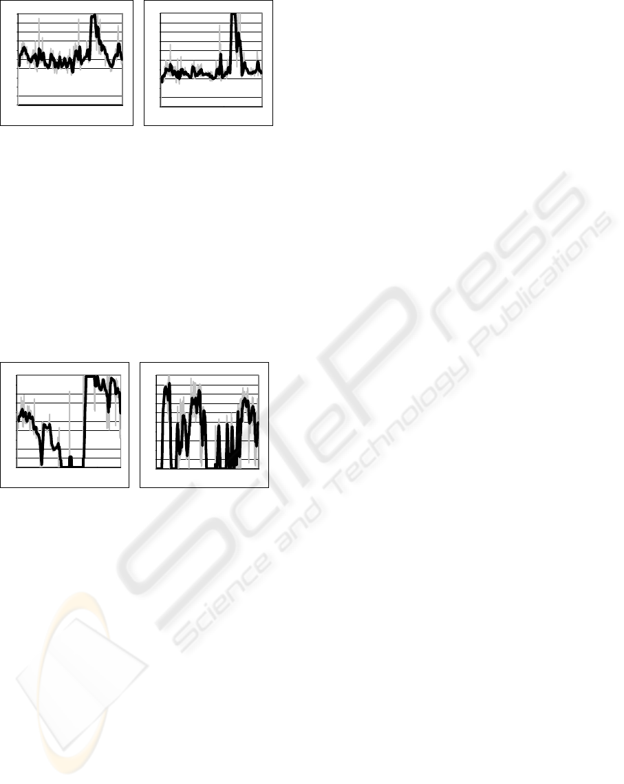
First we show the method of Section 3.1 with 8
direction bins without and with the Markovian
support on Figure 2. Please note, that the Markovian
extension increased the difference between the
anomalous and usual event with approximately 30%.
The main advantage of the GMM method of
Section 3.2 should be the estimation of probabilities
at places where only a very few observations are
available and the adaptation to any directions. The
problem comes with the settings of parameters
(learning rate, weights, directions and variance). The
left of Figure 3 shows the result of the algorithm
using 8 distributions and following the update
procedure of (Stauffer, 1999). In case of the
synthetic video we get slightly worse results than
with the previous method but we should not forget
that the synthetic test video contained only two
typical motion directions (horizontal motion to the
left and to the right). In case of the other videos,
with more motion trajectory directions, we
experienced smaller performance loss.
0
0,1
0,2
0,3
0,4
0,5
0,6
0,7
0,8
0,9
1
220
1
223
4
2267
2
30
0
2
33
3
2
36
6
2399
24
3
2
24
6
5
2498
0
0,1
0,2
0,3
0,4
0,5
0,6
0,7
0,8
0,9
1
2201 2221 2241 2261 2281 2301 2321 2341 2361 2381 2401 2421 2441 2461 2481
Figure 2: Left:
)(U
P
of the most suspicious blob based on
the estimated probabilities for the video “Syn”. The peak
at frame 2500 shows the anomalous motion. Right:
using
),( MU
P
increases the difference between the
unusual event and other local peaks.
The spatial support of segmentation (described in
Section 3.3) can help to eliminate observation noise
but can also filter out small regions of valuable data.
See the right of Figure 3 showing the best results of
the example video.
Two other examples of the algorithm based on
probability segmentation are on Figure 4. Left is
VISAPP 2008 - International Conference on Computer Vision Theory and Applications
680

0
0,1
0,2
0,3
0,4
0,5
0,6
0,7
0,8
0,9
1
2201 2220 2239 2258 2277 2296 2315 2334 2353 2372 2391 2410 2429 2448 2467 2486
0
0,1
0,2
0,3
0,4
0,5
0,6
0,7
0,8
0,9
1
2201 2219 2237 2255 2273 2291 2309 2327 2345 2363 2381 2399 2417 2435 2453 2471 2489
Figure 3: Left:
),( MU
P
of the most suspicious blob based
on the GMM estimation for the video “Syn”. The
difference between usual and unusual events decreased
compared to the previous method. Right: Detection by
segmenting the probability field.
the result of the video where the bicyclist is detected
(“Crossing” sequence) while the right graph shows
the most suspicious blob’s probability in the
“Lanes” video. It is obvious where the bicycle
appears in the last third of the graph while in the
other example the first peak belongs to the people
crossing the street while other smaller peaks belong
to cars touching the centre lines.
0
0,1
0,2
0,3
0,4
0,5
0,6
0,7
0,8
0,9
1
27504 27591 27678 27765 27852 27939 28026 28113 28200 28287 28374 28461 28548 28635 28722 28809 28896 28983
0
0,1
0,2
0,3
0,4
0,5
0,6
0,7
0,8
0,9
1
6501 6607 6716 6821 6932 7044 7155 7267 7381 7493 7605 7711 7822 7930 8039 8151 8267 8377
Figure 4: Left:
),( MU
P
of the most suspicious blob
obtained by segmenting the probability field of the video
“Crossing”. Right: the same for the video “Lanes”.
6 CONCLUSIONS
We considered three pixel-based approaches for the
local representation of motion directions. The
Markovian hypothesis proved to be very useful
giving more discriminating power between unusual
and usual events. The method of Estimated
empirical probability requires the quantization of
motion directions which can reduce the sensitivity in
case of very complex motion fields and makes the
method less sensible for little deviations. Mixture of
Gaussians can reduce the memory requirements and
can maintain arbitrary directions. The traditional
update of model parameters (
Stauffer, 1999) can not
follow the changes in traffic; instead an Expectation
Maximization algorithm should be tested in future.
The Mean-shift segmented probability field
introduces spatial support with some improvements.
All methods run in real-time (@3-15Hz) on a 3GHz
PC considering a 320x240 colour image with
varying frame rate
ACKNOWLEDGEMENTS
The authors would like to thank the help of Attila
Licsár and the support of the GVOP-3.1.1.-2004-05-
0388/3.0 national project.
REFERENCES
E. L. Andrade, S. J. Blunsden, and R. B. Fisher.
Characterisation of optical flow anomalies in
pedestrian traffic. The IEE International Symposium
on Imaging for Crime Prevention and Detection, pp.
73-78, 2005.
J.R. Bergen & R. Hingorani. Hierarchical Motion-Based
Frame Rate Conversion. Technical report, David
Sarnoff Research Center Princeton NJ 08540, 1990.
O. Boiman, M. Irani, Detecting Irregularities in Images
and in Video. International Conference on Computer
Vision (ICCV), Bejing, pp. 462-469, 2005.
M. Brand and V. Kettnaker. Discovery and segmentation
of activities in video. IEEE Trans. Pattern Analysis
and Machine Intelligence, 22(8), pp. 844–851, August
2000.
Anthony R. Dick and Michael J. Brooks. Issues in
Automated Visual Surveillance, International
Conference on Digital Image Computing: Techniques
and Applications (DICTA 2003), Sydney, pp.195-204.
2003.
Bogdan Georgescu, Ilan Shimshoni, and Petert Meer.
Mean shift based clustering in high dimensions: A
texture classification example, 9th International
Conference on Computer Vision, Nice, pp. 456-463,
2003.
Weiming Hu, Tieniu Tan, Liang Wang, and Steve
Maybank. A Survey on Visual Surveillance of Object
Motion and Behaviours, IEEE Transactions on
Systems, Man and Cybernetics, Part C: Applications
and Reviews, Vol 34, Issue 3, pp. 334-352, 2004.
V. Nair and J.J. Clark. Automated visual surveillance
using hidden Markov models. In VI02, pp 88, 2002.
I. Pavlidis, V. Morellas, P. Tsiamyrtzia, and S. Harp.
Urban surveillance systems: from the laboratory to the
commercial world. Proceedings of the IEEE, 89(10),
pp. 1478–1497, 2001.
C. Stauffer and W.E.L. Grimson. Adaptive Background
Mixture Models for Real-time Tracking. CVPR, pp.
246-252, 1999.
ANOMALY DETECTION WITH LOW-LEVEL PROCESSES IN VIDEOS
681