SINGLE-IMAGE 3D RECONSTRUCTION OF BALL VELOCITY

AND SPIN FROM MOTION BLUR

An Experiment in Motion-from-Blur

Giacomo Boracchi, Vincenzo Caglioti and Alessandro Giusti

Dipartimento di Elettronica e Informazione,

Politecnico di Milano, Via Ponzio, 34/5 20133 Milano, Italy

Keywords:

Motion Blur, 3D Motion Reconstruction, Single Image Analysis, Blur Analysis.

Abstract:

We present an algorithm for analyzing a single calibrated image of a ball and for reconstructing its instanta-

neous motion (3D velocity and spin) by exploiting motion blur. We use several state-of-the-art image process-

ing techniques for extracting information from the space-variant blurred image, then robustly integrate such

information in a geometrical model of the 3D motion. We initially handle the simpler case in which the ball

apparent translation is neglegible w.r.t. its spin, then extend the technique to handle the most general motion.

We show extensive experimental results both on synthetic and camera images.

In a broader scenario, we exploit this speciﬁc problem for discussing motivations, advantages and limits of

reconstructing motion from motion blur.

1 INTRODUCTION

In this paper we propose a technique for estimating

the motion of a ball from a single motion blurred

image. We consider the instantaneous ball motion,

which can be described as the composition of 3D

velocity and spin: the proposed technique estimates

both these components by analyzing motion blur.

A more traditional and intuitive method consists

in recovering motion by analyzing successive video

frames: the expected shortcomings of such modus

operandi in realistic operating conditions motivate

our unusual approach. In fact, depending on equip-

ment quality, lighting conditions and ball speed, a

moving ball often results in a blurred image. Fea-

ture matching in successive video frames becomes

very challenging because of motion blur and also be-

cause of repetitive features on the ball surface: this

prevents inter-frame ball spin recovery. Then, it is

worth considering intra-frame information carried by

the motion blur. Our single-image approach has the

further advantage of enabling the use of cheap, high-

resolution consumer digital cameras, which currently

provide a much higher resolution than much more ex-

pensive video cameras. High resolution images are

vital for performing accurate measurements as the

ball usually covers a small part of the image.

We use an alpha matting algorithm (see Sec-

tion 3.1), as a preliminary step before applying a

known technique for estimating the 3D position and

velocity of an uniformly colored ball from a single

blurred image (Boracchi et al., 2007). This allows

us to relax the uniform color assumption and con-

sider textured balls on known background. Once the

ball position and velocity are known, we analyze the

blurred image of the ball textured surface: in particu-

lar, blur is characterized by smears which have vary-

ing direction and extent, resulting from the 3D motion

of the ball surface. We estimate spin by analyzing

such smears within small image patches, and by inte-

grating them on a geometrical 3D model of the ball.

The blur model derived from the 3D ball motion is

presented in Section 2, while in Section 3 we brieﬂy

recall the image analysis algorithms used. The pro-

posed technique is described in Section 4. Section 5

presents experimental results and Section 6 summa-

rizes the work and presents future research directions.

1.1 Related Works

Given a single blurred image, the most treated prob-

lem in literature is the estimation of the point spread

function (PSF) that corrupted the image (Fergus et al.,

2006; Levin, 2007; Jia, 2007), usually with the pur-

pose of image restoration (deblurring).

Our work, on the contrary, takes advantage of mo-

tion blur for performing measurements on the im-

aged scene. Several other works follow a similar ap-

proach, such as (Klein and Drummond, 2005), which

describes a visual gyroscope based on rotational blur

Boracchi G., Caglioti V. and Giusti A. (2008).

SINGLE-IMAGE 3D RECONSTRUCTION OF BALL VELOCITY AND SPIN FROM MOTION BLUR - An Experiment in Motion-from-Blur.

In Proceedings of the Third International Conference on Computer Vision Theory and Applications, pages 22-29

DOI: 10.5220/0001088000220029

 SciTePress

Figure 1: Some blurred ball images. Leftmost images are textureless, so their spin can not be recovered. Central images show

textured balls whose spin component dominates the apparent translation. Rightmost images are the most complete case we

handle, showing a signiﬁcant amount of apparent translation and spin; note that the ball contours also appear blurred in this

situation, whereas they are sharp in the spin-only case.

analysis, or (Levin et al., 2007), which estimates the

scene depth map from an image acquired with a coded

aperture camera. Also, (Rekleitis, 1996) proposes to

estimate the optical ﬂow from a single blurred im-

age. A ball speed measurement method based on a

blurred image has been proposed in (Lin and Chang,

2005). This assumes a simpliﬁed geometrical model

that originates space-invariant blur and prevents the

estimation of 3D motions and spin.

On the other hand, the problem of estimating the

motion of a ball in the 3D space has been extensively

treated in video tracking literature (Gopal Pingali and

Jean, 2000; J Ren and Xu, 2004; Jonathan Rubin

and Stevens, 2005). These methods assume the ball

visible from multiple synchronized cameras, in order

to triangulate the ball position in the corresponding

frames. In (Reid and North, 1998) a method is pro-

posed for reconstructing the ball 3D position and mo-

tion from a video sequence by analyzing its shadow.

In (Kim et al., 1998; Ohno et al., 2000), a physics-

based approach is adopted, to estimate the parameters

of a parabolic trajectory.

Recently, some methods for estimating the 3D

ball trajectory from image blur have been pro-

posed (Caglioti and Giusti, 2006; Boracchi et al.,

2007). However, these methods assume an uniformly-

colored ball, and do not recover spin.

2 PROBLEM FORMULATION

Let S be a freely moving ball centered in C, whose

radius R is known

, imaged by a calibrated camera.

We assume that during the exposure time T the ball

if the radius is not known, the whole reconstruction can

be performed up to a scale factor

motion is deﬁned by the composition of two factors:

• a linear translation with uniform velocity, u. The

translation distance during the exposure is there-

fore T · u.

• the spin around a rotation axis a passing through

C, with angular speed ω. The rotation angle which

occurs during the exposure is therefore T ·ω.

From the ball localization technique (Boracchi

et al., 2007) we inherit the constraint that the ball

projections at the beginning and at the end of the ex-

posure signiﬁcantly overlap. Moreover, in order to

recover the rotation axis and speed, we also require

that spin is not too fast nor too slow w.r.t. the ex-

posure time: π/50 < ω · T < π/2. In practice, these

constraints allow us to use an exposure time 5 ÷ 10

times longer than the exposure time which would give

a sharp image.

Our goal is to estimate the ball spin (both a and ω),

velocity u, and initial position by analyzing a single

blurred image.

We assume that the blur on pixels depicting the

ball is only due to ball motion. In practice, this can be

achieved if the ball is in focus and the camera is still.

Therefore the image formation model, on which our

analysis is based, can be described as follows.

2.1 Blurred Image Formation

Let Z be the blurred image that depicts the mov-

ing ball and let [0,T ] be the exposure interval. The

blurred image Z can be modeled as the integration of

inﬁnitely many (sharp) sub-images I

,t ∈ [0, T ], each

depicting the ball in a different 3D position and spin

angle (see Figure 2):

Z(x) =

(x)dt + η(x), x ∈ X. (1)

SINGLE-IMAGE 3D RECONSTRUCTION OF BALL VELOCITY AND SPIN FROM MOTION BLUR - An Experiment

in Motion-from-Blur

Figure 2: Blurred image formation model. The blurred im-

age Z is obtained as the temporal integration of many still

images I

. The alpha map α of the blurred ball represents

the motion of the object’s contours and is used for recover-

ing the translational motion component.

Where x represents the 2D image coordinates, I

(x) is

the light intensity that reaches the pixel x at time t,

and η ∼ N(0,σ

) is white gaussian noise.

The ball apparent contours γ

,t ∈ [0,T ] vary de-

pending on translation only. Note that each apparent

contour γ

is an ellipse and that, in each sub-image

, γ

may have a different position and also a dif-

ferent shape because of perspective effects (Boracchi

et al., 2007). On the contrary, the spin does not affect

,t ∈ [0,T ]. In our reconstruction procedure, we will

exploit the fact that the alpha map α of the blurred ball

only depends on variations in γ

, and is not affected

by spin. The ball spin, combined with the translation,

changes the depicted ball surface in each sub-image I

and obviously the appearance of the ball in Z.

2.2 Blur on the Ball Surface

We treat the blur on the ball surface as locally space

invariant (Bertero and Boccacci, 1998). In particular

we approximate the blur in a small image region as

the convolution of the sub-image I

with a PSF having

vectorial support and constant value on it. Hence for

any pixel x

belonging to the ball image, we consider

a neighborhood U

of x

and a PSF h

such that

Z(x) =

(x − s)I

(s)ds + η(x) , ∀x ∈ U

(2)

The PSF h

is identiﬁed by two parameters, the direc-

tion θ

and the extent l

3 IMAGE ANALYSIS

The proposed algorithm exploits two blur analysis

techniques in order to separately handle the effects of

ball translation and ball spin. The ball position and

velocity u in 3D space are obtained by combining an

alpha matting technique with the method presented in

(Boracchi et al., 2007). The ball spin is computed by

estimating the blur parameters within small regions

on the ball image.

3.1 Alpha Matting

Alpha matting techniques have been recently applied

to motion blurred images with different purposes, in-

cluding PSF estimation (Jia, 2007) and blurred smear

interpretation (Caglioti and Giusti, 2007). As shown

in (Giusti and Caglioti, ), by applying alpha matting

to the motion-blurred image of an object we obtain a

meaningful separation between the motion of the ob-

ject’s boundaries (alpha map) and the actual blurred

image of the object (color map).

As we described in the previous section, in this

scenario the alpha map of a blurred ball is not in-

ﬂuenced by the spin but only by the translation: in

practice, the alpha map is the image we would ob-

tain if the background was black and the ball had a

uniformly-white projection. Therefore the alpha map

of the blurred ball can be used to estimate the ball po-

sition and displacement vector T · u according to the

technique presented in (Boracchi et al., 2007), even

when the ball surface is textured.

On the contrary, the color map only shows the

blurred ball image, as if it was captured over a black

background. In the following sections, the color map

will be analyzed in order to recover the ball spin.

In the general case, the matting problem is under-

constrained, even if the background is known. Still, in

literature many algorithms have been proposed: some

of them (Smith and Blinn, 1996; Mishima, 1993)

require a speciﬁc background (blue screen matting),

whereas others, with minimal user assistance, handle

unknown backgrounds (natural image matting) and

large zones of mixed pixels (0 < α < 1). Although

none is explicitly designed for the interpretation of

motion blurred images, we can get satisfactory results

in our peculiar setting. In this context, however, we

adopted (Giusti and Caglioti, ), a fast and exact alpha

matting algorithm, very suited to sport environments

where its requirements on the background and fore-

ground colors are often met.

3.2 Blur Analysis

As mentioned in Section 2.2, we approximate the blur

as locally shift invariant, produced by a convolution

with a PSF having vector-like support. We estimate

the blur direction and extent separately on N image

VISAPP 2008 - International Conference on Computer Vision Theory and Applications

Figure 3: A synthetic image of a spinning golf ball. U

neighborhoods and recovered blur directions and extents are

shown. Each segment b

represents the blur parameters θ

within the region.

regions U

i = 1,..,N containing pixels which have

been covered by the ball projection during the entire

exposure time, i.e. α(x) = 1 ∀x ∈ U

, i = 1, ..,N.

In particular we apply the method proposed in

(Yitzhaky and Kopeika, 1996) and we estimate the

blur direction as the direction having minimum

derivative energy. This is motivated by the fact that

most of image details along the blur direction are

smoothed by blur. After estimating the blur direc-

tion, the blur extent is obtained from the distance be-

tween two negative peaks in the autocorrelation of di-

rectional derivatives along the blur direction. Figure 3

shows some square regions used for blur analysis.

Other techniques for estimating the local blur di-

rections may be used: for example, when the ball tex-

ture contains corners (like in most football balls), the

method presented in (Boracchi and Caglioti, 2007)

can be applied. Alternatively, blurred smears of

strong features can be highlighted by applying the ﬁl-

tering techniques in (Caglioti and Giusti, 2007).

4 RECONSTRUCTION

TECHNIQUE

For clarity purposes we illustrate the proposed tech-

nique ﬁrst in the simpler case, where blur is due to

ball spin only. Then, in Section 4.2.1 we cope with

the most general case where the ball simultaneously

translates and spins.

4.1 Null Translation

Let assume that during the exposure the ball does not

translate, i.e. u = 0, so that in the blurred image the

ball apparent contour is sharp. The ball apparent con-

tour γ is an ellipse and it allows us to localize the ball

in the 3D space by means of the camera calibration

parameters and knowledge of the ball radius. Points

belonging to γ are easily found in the image either by

ordinary background subtraction or using edge points

in the alpha matte. We extract γ by ﬁtting an ellipse to

such points, enforcing the projective constraint of be-

ing the image of a sphere captured from the calibrated

camera.

Then, the blur is analyzed within N regions

, i = 1,.., N contained inside γ. In order to avoid

uniform-color areas, we select such regions around

local maxima x

,i = 1,..,N of the Harris corner mea-

sure (Harris and Stephens, 1988). For each of these

points, a local blur direction θ

is obtained using

method presented in (Yitzhaky and Kopeika, 1996).

Such directions are now exploited in order to re-

cover the 3D motions v

of the ball surface at points

corresponding to each of the regions. Since the cam-

era is calibrated and we know the 3D position of the

sphere S, we can backproject each pixel x

on the

sphere surface. Let X

be the intersection point, clos-

est to the camera, between the viewing ray of x

and

sphere S: the 3D motion direction of the ball surface

at X

is described by an unit vector v

(see Figure 4

left). More precisely, let π

be the plane tangent to S

at X

: then, v

is found as the direction of the intersec-

tion between π

and the viewing plane of the image

line passing through x

and having direction θ

As shown in Figure 4 (left), all the vectors

i = 1,..,N must lie on the same plane, orthogo-

nal to the rotation axis a. Then, let W = [v

|..|v

be the matrix having vectors v

as columns. The direc-

tion of a is found as the direction of the eigenvector

associated to the smallest of W ’s eigenvalues. This

estimate is reﬁned by iterating the procedure after re-

moving the v

vectors that deviate too much from the

plane orthogonal to a (outliers).

Note that, when the ball is not translating, the ball

apparent contour γ is sharp and in this case it is eas-

ily localized by ﬁtting an ellipse to image edge points

(possily after background subtraction) or by using a

generalized Hough transform, without need of alpha

matting.

Although the rotation axis can be recovered ex-

ploiting θ

directions only, in order to estimate the an-

gular speed we need to consider also the blur length

estimated within regions U

. Each of these extents

represents the length of the trajectory (assumed rec-

tilinear) that the feature traveled in the image during

the exposure. For each feature, a starting point b

and

ending point e

are determined in the image as

= x

−



cosθ

sinθ



= x



cosθ

sinθ



(3)

and backprojected on the sphere surface S to points

and E

, respectively. We then compute the dihe-

SINGLE-IMAGE 3D RECONSTRUCTION OF BALL VELOCITY AND SPIN FROM MOTION BLUR - An Experiment

in Motion-from-Blur

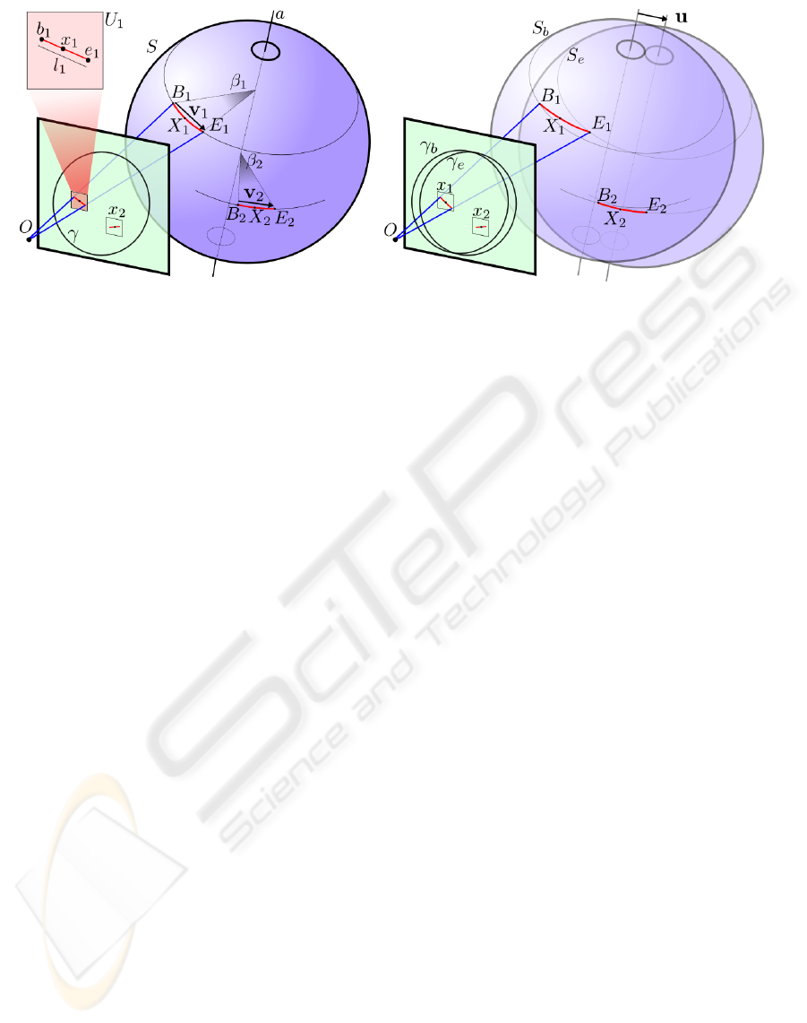
Figure 4: Left: reconstruction geometry for zero translation. Right: reconstruction for full motion case.

dral angle β

between two planes, one containing a

and B

, the other containing a and E

. Such angles

are computed only for those estimates not previously

discarded as outliers. The spin angle is estimated as

the median of the β

angles. If the exposure time T

is known, the spin angular speed ω immediately fol-

lows.

4.2 Combining Ball Spin and Ball

Translation

If the ball contour changes during the exposure, the

procedure is modiﬁed as follows (see Figure 4 right).

At ﬁrst, the image is decomposed in an alpha map

and a color map, as described in Section 3.1. The

alpha map is used to recover the ball apparent con-

tours at the beginning (γ

) and end (γ

) of the expo-

sure. These are determined using the method pre-

sented in (Boracchi et al., 2007), which returns two

spheres S

and S

having centers C

and C

respec-

tively. This reconstructs the ball position and transla-

tion during the exposure and, when the exposure time

T is known, also the ball velocity. Blur is then ana-

lyzed within regions U

, i = 1,..,N of the color map

whose pixels x satisfy the condition α(x) = 1, i.e. pix-

els which have been covered by the ball during the

whole exposure. For each U

, image points b

and e

are returned, as described in Section 4.1.

In this case, backprojecting the blur direction on

the sphere is meaningless, since blur is caused by si-

multaneous translation and spin. Therefore, the view-

ing ray of b

is intersected with S

, which identiﬁes a

3D point B

and similarly, e

is backprojected on S

ﬁnd E

(see Figure 4 (right)).

For each region, the 3D vector

= (E

− B

) − (C

−C

) (4)

represents the 3D motion of the ball surface at the

corresponding point, due to the spin component only.

The spin axis a and angular velocity ω are now esti-

mated as in the previous case.

4.2.1 The Orientation Problem

Each motion recovered from blur analysis has an ori-

entation ambiguity. This holds for the ball motion,

and also for the blur directions estimates θ

. The

ambiguity is explained by Equation (1) where the

blurred image is given by an integration of several

sub-images: obviously, information about the order

of sub-images is lost.

In the ball localization step we arbitrarily choose

which of the two found ellipses is γ

, representing the

ball at the beginning of the exposure, and which is

. But when each blurred feature x

is considered

and its endpoints b

, e

identiﬁed, there is no way to

determine which corresponds to the feature location

at the beginning of the exposure. Now the choice is

not arbitrary since each must be backprojected to the

correct sphere (S

and S

, respectively).

We propose the following possible criteria for

solving the problem:

• if translation dominates spin, blurred features

should be oriented in the direction of the trans-

lational motion;

• blur orientations in nearby regions should be sim-

ilar;

• for features having one endpoint outside the inter-

section area between γ

and γ

only one orienta-

tion is consistent.

Another solution is computing the two possible vec-

tors v

and v

for each feature, then using a RANSAC-

like technique to discard the wrong ones as outliers.

VISAPP 2008 - International Conference on Computer Vision Theory and Applications

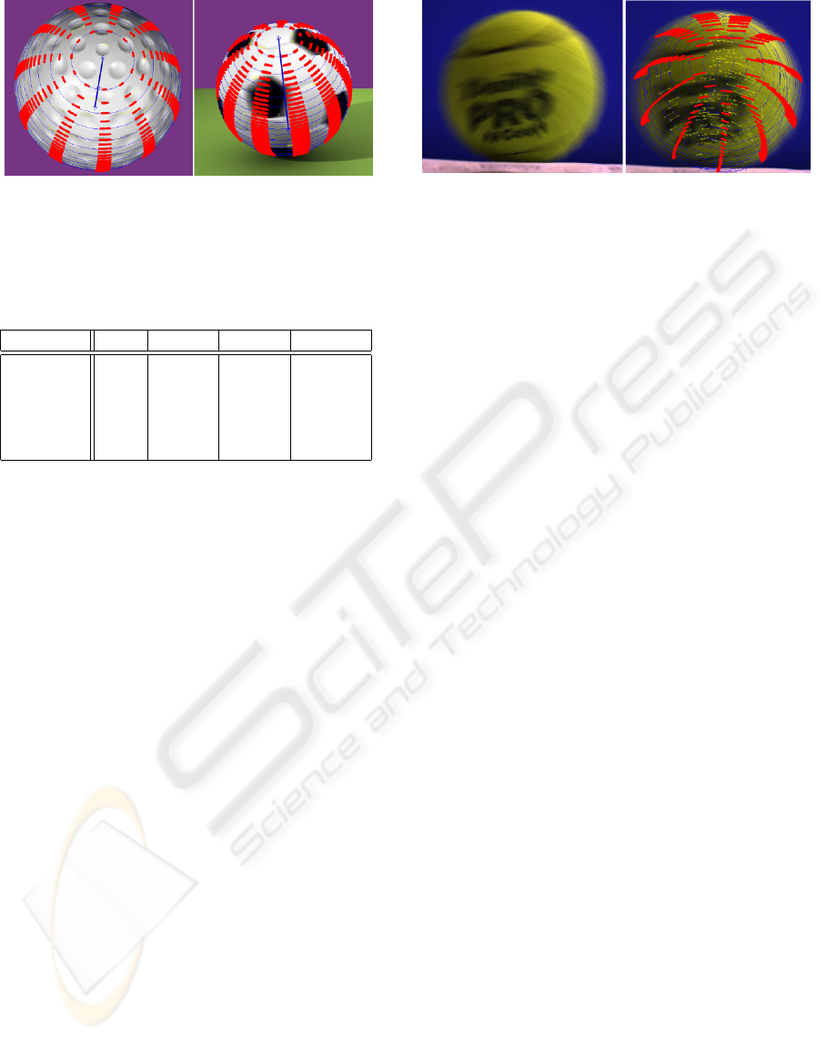
Figure 5: Reconstruction results on two synthetic images

(spin only).

Table 1: Mean relative error in ω estimation, expressed as a

percentage w.r.t the true value of ω. Columns where σ > 0

shows the average over ten noise realizations. Image data is

in the 0 ÷ 255 range.

ω · T \ σ 0 1 2 3

5.00 4.31 4.6222 5.0641 3.9401

6.25 2.26 2.5562 4.7898 4.3915

7.50 2.40 3.1353 2.7236 2.0544

8.75 0.75 1.5163 2.9408 5.0431

10.00 2.15 3.3975 5.3916 11.3800

5 EXPERIMENTS

We validated our technique on both synthetic and

camera images.

Each synthetic image has been generated accord-

ing to (1), by using the Blender 3D modeler for ren-

dering hundreds of sharp frames each depicting the

moving ball at a different t belonging to the expo-

sure interval [0,T ]. Each frame corresponds to a sub-

image I

, and all these sub-images are averaged to-

gether. We generated images with varying, known

spin amount ω · T in the 1

◦

÷ 20

◦

range, both in the

spin-only and in the spin plus translation cases. Sev-

eral scenarios (some are shown in Figures 5 and 7)

have been rendered with different spin axes w.r.t to the

camera. Some of our test cases use a plain texture for

the ball, whereas others feature a realistic ball surface

with 3D details such as bumps and seams, and spec-

ular shading; this simulates difﬁcult operating condi-

tions, in which the ball appearance under motion is

not easily deﬁned.

Table 1 shows algorithm performance for ω es-

timation in an 800x600 image also accounting for

noise. Figure 7 shows some of the synthetic images

we used. The algorithm accuracy is reduced when the

ball spin is too low as the small ball resolution does

not allow reliable estimates in small regions U

. Con-

sidered regions are disk shaped, having radius varying

between 30-45 pixels according to the noise standard

deviation σ, estimated using (Donoho and Johnstone,

Figure 6: A real image (tennis ball) spinning and translat-

ing, and reconstructed motion (right). Note complex motion

of points on the ball surface due to simultanous spin and

translation: red stripes show reconstructed motion, and cor-

rectly interpret the observed blur. Since the ball was rolling

on a table (bottom of the image), features on the bottom of

the ball are correctly estimated as still, and the rotation axis

as coplanar with the table.

1994).

Both in synthetic and camera images, the blur es-

timates show a variable percentage of outliers (5% ÷

50%), which are correctly discarded in most cases.

Outliers are more frequent in noisy images, with

smaller spin amounts and where the ball texture

shows strong, straight edges.

We found that, in general, the estimation of blur

extents l

is much more error-prone than the estima-

tion of blur angles θ

, without signiﬁcant differences

between real and synthetic images. Together with the

orientation problem (see Section 4.2.1), this makes

the analysis of the general motion case much more

challenging than the spin-only case (where the extents

are only used to estimate ω · T ).

6 DISCUSSION, CONCLUSIONS

AND ONGOING WORKS

We propose a technique for reconstructing the veloc-

ity and spin of a moving ball from a single motion-

blurred image, highlighting advantages and disadvan-

tages of the approach. Our tests show very promising

results, both in synthetic and real images, especially

if the ball’s apparent translation during the exposure

is negligible (i.e. the ball contours are sharp). This

scenario, which is not unusual in practice, has several

important practical advantages such as no need of al-

pha matting, limited reliance on the estimation of blur

lengths – which we have found to be quite unreliable

– and irrelevance of the orientation problem.

In a broader view, our technique solves a nontriv-

ial motion estimation problem from the motion blur

in a single image. Although unusual, this approach

may result successful in situations where traditional

SINGLE-IMAGE 3D RECONSTRUCTION OF BALL VELOCITY AND SPIN FROM MOTION BLUR - An Experiment

in Motion-from-Blur

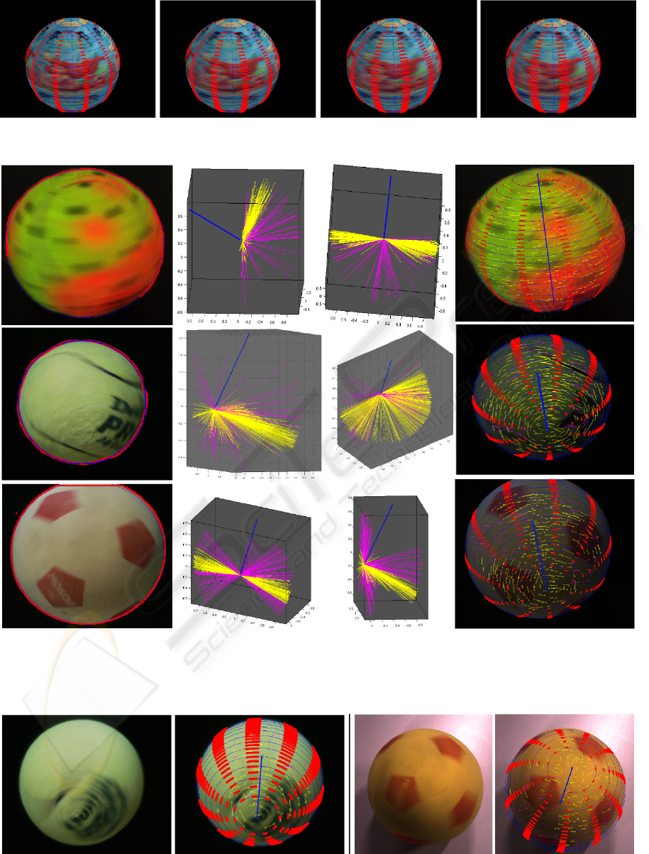
Figure 7: Synthetic image of textured ball at different ω values. From left to right ω · T = 5

◦

;6.875

◦

;8.125

◦

;10

◦

Figure 8: Real images (spin only). Central columns shows axis (blue) and v

directions from different viewpoints: yellow

ones are inliers, magenta are outliers. Corresponding blur estimates are shown in the rightmost image as yellow segments.

Reconstructed spin axes and speeds correctly explain the blurred image: for example, the spin axis passes through the sharpest

parts of the ball image.

Figure 9: Other real images, and reconstructed motions (spin only). Display colors are the same as in previous ﬁgures.

VISAPP 2008 - International Conference on Computer Vision Theory and Applications

video-based methods fail; target applications include

training support and match analysis in sport environ-

ments.

Other than further improving our software toward

a more robust implementation, we are currently in-

vestigating the practical possibility of estimating spin

axis and velocity without the need of blur extents.

Moreover, we are testing other techniques for blur es-

timation and alpha matting.

REFERENCES

Bertero, M. and Boccacci, P. (1998). Introduction to Inverse

Problems in Imaging. Institute of Physics Publishing.

Boracchi, G. and Caglioti, V. (2007). Corner displacement

from motion blur. In proc. of ICIAP 2007 Conference.

Boracchi, G., Caglioti, V., and Giusti, A. (2007). Ball po-

sition and motion reconstruction from blur in a sin-

gle perspective image. In Inproceedings of ICIAP

2007,Modena.

Caglioti, V. and Giusti, A. (2006). Ball trajectory recon-

struction from a single long-exposure perspective im-

age. In Proc. of Workshop on Computer Vision Based

Analysis in Sport Environments (CVBASE).

Caglioti, V. and Giusti, A. (2007). On the apparent trans-

parency of a motion blurred object. In Proc. of ICCV

workshop on Photometric Analysis in Computer Vi-

sion (PACV) 2007.

Donoho, D. L. and Johnstone, I. M. (1994). Ideal spa-

tial adaptation by wavelet shrinkage. Biometrika,

81(3):425–455.

Fergus, R., Singh, B., Hertzmann, A., Roweis, S. T., and

Freeman, W. T. (2006). Removing camera shake from

a single photograph. In ACM SIGGRAPH 2006 Pa-

pers.

Giusti, A. and Caglioti, V. Isolating motion and color in a

motion blurred image. In Proc. of BMVC 2007.

Gopal Pingali, A. O. and Jean, Y. (2000). Ball tracking

and virtual replays for innovative tennis broadcasts.

In proc. of ICPR 2000 Conference, page 4152, Wash-

ington, DC, USA. IEEE Computer Society.

Harris, C. and Stephens, M. (1988). A combined corner and

edge detector. In Proceedings of the 4th Alvey Vision

Conference,, pages 147–151.

J Ren, J. Orwell, G. J. and Xu, M. (2004). A general frame-

work for 3d soccer ball estimation and tracking. In

Proc. of ICIP 2004 Conference.

Jia, J. (2007). Single image motion deblurring using trans-

parency. In Inproceedings of CVPR 2007, Minneapo-

lis.

Jonathan Rubin, Burkhard C. Wuensche, L. C. and Stevens,

C. (2005). Computer vision for low cost 3-d golf ball

and club tracking. In Proc. of Image and Vision Com-

puting New Zealand.

Kim, T., Seo, Y., and Hong, K.-S. (1998). Physics-based

3d position analysis of a soccer ball from monocular

image sequences. In proc of ICCV 1998 Conference,

pages 721–726.

Klein, G. and Drummond, T. (2005). A single-frame visual

gyroscope. In Proc. British Machine Vision Confer-

ence (BMVC’05), volume 2, pages 529–538, Oxford.

BMVA.

Levin, A. (2007). Blind motion deblurring using image

statistics. In Sch

olkopf, B., Platt, J., and Hoffman,

T., editors, Advances in Neural Information Process-

ing Systems 19. MIT Press, Cambridge, MA.

Levin, A., Fergus, R., Durand, F., and Freeman, W. T.

(2007). Image and depth from a conventional camera

with a coded aperture. ACM Trans. Graph., 26(3):70.

Lin, H.-Y. and Chang, C.-H. (2005). Automatic speed mea-

surements of spherical objects using an off-the-shelf

digital camera. In Mechatronics, 2005. ICM ’05. IEEE

International Conference on, pages 66–71.

Mishima, Y. (1993). Soft edge chroma-key generation

based upon hexoctahedral color space. U.S. Patent

5,355,174.

Ohno, Y., Miura, J., and Shirai, Y. (2000). Tracking players

and estimation of the 3d position of a ball in soccer

games. In ICPR, pages 1145–1148.

Reid, I. D. and North, A. (1998). 3d trajectories from a

single viewpoint using shadows. In proc. of BMVC

1998 Conference.

Rekleitis, I. M. (1996). Steerable ﬁlters and cepstral anal-

ysis for optical ﬂow calculation from a single blurred

image. In Vision Interface, pages 159–166, Toronto.

Smith, A. R. and Blinn, J. F. (1996). Blue screen matting.

In SIGGRAPH ’96: Proc. of the 23rd annual con-

ference on Computer graphics and interactive tech-

niques, pages 259–268.

Yitzhaky, Y. and Kopeika, N. S. (1996). Identiﬁcation of

blur parameters from motion-blurred images. In Proc.

SPIE Vol. 2847, pages 270–280.

SINGLE-IMAGE 3D RECONSTRUCTION OF BALL VELOCITY AND SPIN FROM MOTION BLUR - An Experiment

in Motion-from-Blur