FACIAL EXPRESSION RECOGNITION USING ACTIVE

APPEARANCE MODELS

Pedro Martins, Joana Sampaio, Jorge Batista

∗

ISR-Institute of Systems and Robotics, Dep. of Electrical Engineering and Computers

FCTUC-University of Coimbra, Coimbra, Portugal

Keywords:

Active appearance models (AAM), Linear discriminant analysis (LDA), Facial expression recognition.

Abstract:

A framework for automatic facial expression recognition combining Active Appearance Model (AAM) and

Linear Discriminant Analysis (LDA) is proposed. Seven different expressions of several subjects, representing

the neutral face and the facial emotions of happiness, sadness, surprise, anger, fear and disgust were analysed.

The proposed solution starts by describing the human face by an AAM model, projecting the appearance

results to a Fisherspace using LDA to emphasize the different expression categories. Finaly the performed

classiﬁcation is based on malahanobis distance.

1 INTRODUCTION

Facial expressions recognition plays an important role

in human communication since has more inﬂuence

than simpler audio information. Psychology studies

(T. Dalgleish, 1999) describe that there are six basic

emotions universally recognized: joy, sadness, sur-

prise, fear, anger and disgust. Notice that, these ex-

pressions are also compatible with MPEG-4 norm.

Clearly, in order to extract facial information from

one image we need to solve ﬁrst the problem of ﬁnd-

ing the face on it. Traditionally, there are two different

ways to approach this problem. Anthropometric fea-

ture extraction (Batista, 2007) based on detection of

facial characteristics such as eyes, eyebrows, mouth

and nose, or using appearance based methods. The

last one, is preferable since it is able to extract rel-

evant face information without background interfer-

ence and describes facial characteristics in a reduced

model. Our work on facial expressions recognition

belongs to the appearance based approaches.

Appearence-based face recognition involves im-

age preprocessing and the use of statiscal redundancy

reduction for compact coding. To synthesize a com-

plete image face, both shape and textute are modelled.

The AAM represents both shape and texture varia-

tions observed in a training image set and the corre-

lations between them. Supervised dimension reduc-

∗

This work was funded by FCT Project POSI/EEA-

SRI/61150/2004

tion use the knowledge of class structure and the use

of multi-linear models allow low-dimensional repre-

sentations which account for variations in geometry,

orientation and illumination.

In statistical supervised learning, Linear Discrim-

inant Analysis (Peter N. Belhumeur and Kriegman,

1997) is a classical solution that ﬁnds the basis vec-

tors maximizing the interclass distances while mini-

mizing the intraclass distances. Linear discriminant

analysis is performed in order to extract the most dis-

criminant features which maximizes class seperabil-

ity. The discriminating power of the appearance pa-

rameters (AAM) is analysed when projected in Fish-

erspace and the degree of similarity is measured in

that subspace using Mahalanobis distances. A series

of experiments where conducted on a set of unknown

images showing the faces of different subjects with

facial expressions ranging neutral to intensely expres-

sive.

This paper is organised as follows: section 2 gives

a brief introduction to the standard ActiveAppearance

Models (AAM) theory, section 3 describes the facial

recognition methodology used, section 4 shows ex-

perimental results and section 5 discusses the results.

123

Martins P., Sampaio J. and Batista J. (2008).

FACIAL EXPRESSION RECOGNITION USING ACTIVE APPEARANCE MODELS.

In Proceedings of the Third International Conference on Computer Vision Theory and Applications, pages 123-129

DOI: 10.5220/0001088701230129

 SciTePress

2 ACTIVE APPEARANCE

MODELS

AAM is a statistical based segmentation method,

where the variability of shape and texture is captured

from the dataset. Building such a model allows the

generation of new instances with photorealistic qual-

ity. In the search phase the model is adjusted to

the target image by minimizing the texture residual.

For futher details refer to (T.F.Cootes and C.J.Taylor,

2001).

2.1 Shape Model

The shape is deﬁned as the quality of a conﬁguration

of points which is invariant under Euclidian Similar-

ity transformations (T.F.Cootes and C.J.Taylor, 2004).

This landmark points are selected to match borders,

vertices, proﬁle points, corners or other features that

describe the shape.

The representation used for a single n-point shape

is a 2n vector given by:

x = (x

,...,x

n−1

)

(1)

With N shape annotations, follows a statistical

analysis where the shapes are previously aligned to a

common mean shape using a Generalised Procrustes

Analysis (GPA) removing location, scale and rotation

efects. Optionaly, we could project the shape distri-

bution into the tangent plane, but omitting this pro-

jection leads to very small changes (Stegmann and

Gomez, 2002).

Applying a Principal Components Analisys

(PCA), we can model the statistical variation with:

x = x+ Φ

(2)

where new shapes x, are synthesised by deforming

the mean shape, x, using a weighted linear combina-

tion of eigenvectors of the covariance matrix, Φ

. b

is a vector of shape parameters which represents the

weights. Φ

holds the t

most important eigenvectors

that explain a user deﬁned variance.

2.2 Texture Model

For m pixels sampled, the texture is represented by

the vector:

g = [g

,...,g

m−1

]

(3)

Building a statistical texture model, requires

warping each training image so that the control points

match those of the mean shape. In order to prevent

holes, the texture mapping is performed using the re-

verse map with bilinear interpolation correction.

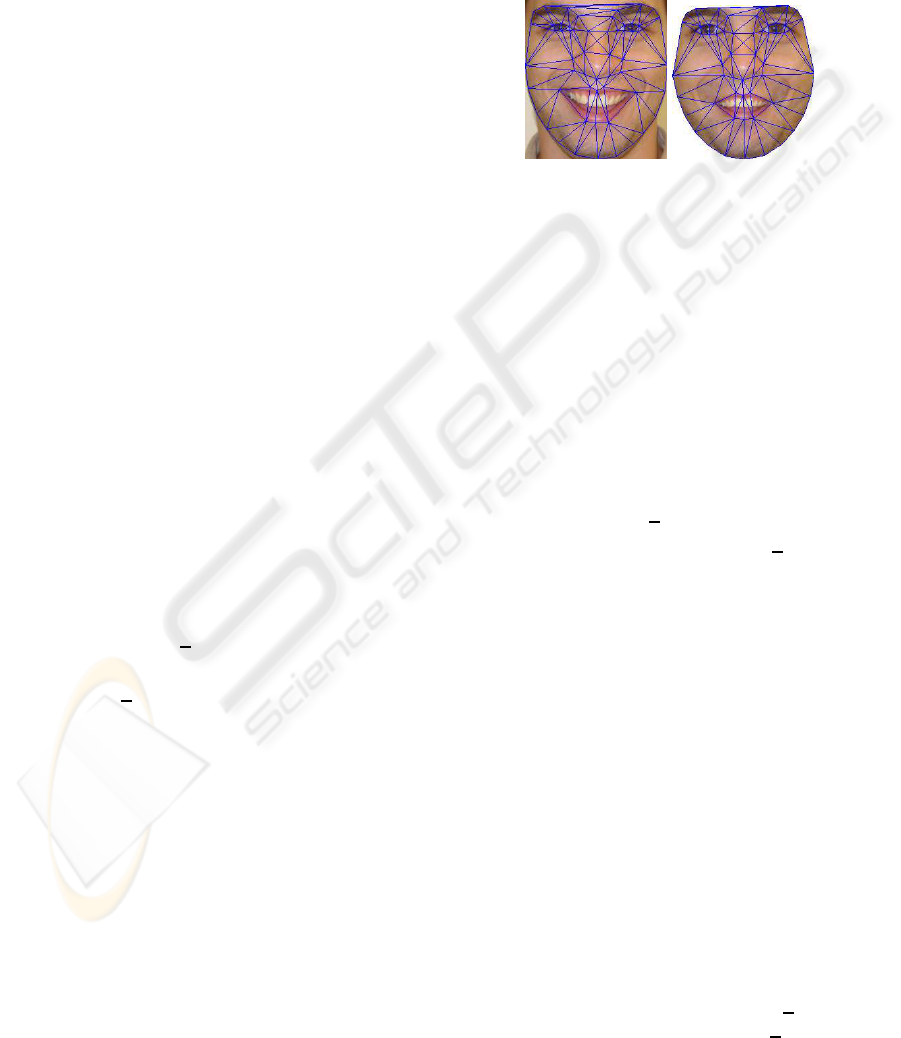
The texture mapping is performed, using a piece-

wise afﬁne warp, i.e. partitioning the convex hull of

the mean shape by a set of triangles using the De-

launay triangulation. Each pixel inside a triangle is

mapped into the correspondent triangle in the mean

shape using barycentric coordinates, see ﬁgure 1.

(a) Original (b) Warped texture

Figure 1: Texture mapping example.

This procedure removes differences in texture due

shape changes, establishing a common texture refer-

ence frame.

To reduce the inﬂuence of global lighting variation

a scaling, α and offset, β is applied

norm

= (g

− β.1)/α (4)

After the normalization we get g

norm

.1 = 0 and

norm

| = 1.

A texture model can be obtained by applying a

PCA on the normalized textures:

g = g+ Φ

(5)

where g is the synthesized texture, g is the mean

texture, Φ

contains the t

highest covariance texture

eigenvectors and b

is a vector of texture parameters.

Another possible solution to reduce the effects of

differences in ilumination is to perform a histogram

equalization independently in each of the three color

channels (G. Finlayson and Tian, 2005).

Similarly to shape analysis, PCA is conducted in

texture data to reduce dimensionality and data redun-

dacy. Since the number of dimensions is greater than

the number of samples (m >> N) it is used a low-

memory PCA.

2.3 Combined Model

The shape and texture from any training example is

described by the parameters b

and b

. To remove

correlations between shape and texture model param-

eters a third PCA is performed to the following data:

b =







(x− x)

(g−g)



(6)

VISAPP 2008 - International Conference on Computer Vision Theory and Applications

124

where W

is a diagonal matrix of weights that

measures the unit difference between shape and tex-

ture parameters. A simple estimate for W

is to

weight uniformly with ratio, r, of the total variance

in texture and shape, i.e. r =

∑

. Then

= rI (Stegmann, 2000).

As result, using again a PCA, Φ

holds the t

high-

est eigen vectors, and we obtain the combined model.

b = Φ

c (7)

Due the linear nature for the model, is possible to

express shape, x, and texture, g, using the combined

model by:

x = x+ Φ

−1

c,s

c (8)

g = g+ Φ

c,g

c (9)

where





(10)

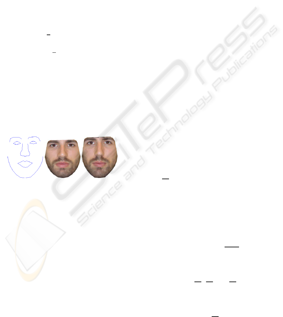
c is a vector of appearance controling both shape

and texture. One AAM instance is built by generating

the texture in the normalized frame using eq. 9 and

warping-it to the control points given by eq. 8. See

ﬁgure 2.

(a) Shape con-

trol points

(b) Texture

in normalized

frame

instance

Figure 2: Building a AAM instance.

2.4 Model Training

An AAM search can be treated as an optimiza-

tion problem, where the texture difference between

a model instace and a target image is minimized,

image

− I

model

updating the appearance parameters

c and pose.

Apparently, this could be a hard optimazation

problem, but we can learn how to solve this class of

ploblems, learning how the model behaves due pa-

rameters change, i.e. learning ofﬂine the relation be-

tween the texture residual and the correspondent pa-

rameters error.

Additionally, are considered the similarity param-

eters for represent the 2D pose. To mantain linear-

ity and keep the identity transformation at zero, these

pose parameters are redeﬁned to: t = (s

)

where s

= (scos(θ) − 1), s

= ssin(θ) represents a

combined scale, s, and rotation, θ. The remaining pa-

rameters t

and t

are the usual translations.

Now the complete model parameters, p, (a t

+ 4 vector) are given by:

p = (c

)

(11)

The initial AAM formulation uses the multivariate

linear regression aproach over the set of training tex-

ture residuals, δg, and the correspondent model per-

tubations, δp. The goal is to get the optimal predition

matrix, in the least square sense, satisfying the linear

relation:

δp = Rδg (12)

Solving eq. 12 involves perform a set s experi-

ences, building the residuals matrices (P holds by col-

uns model parameters pertubations and G holds cor-

respondent texture residuals):

P = RG (13)

In AAM its safe to say that m >> t

> t

, so one

possible solution of eq. 13 can be obtained by Prin-

cipal Component Regression (PCR) projecting the

large matrix G into a k−dimensional subspace, where

k ≥ t

which captures the major part of the variation.

Later (T.F.Cootes and C.J.Taylor, 2001) it was

suggested a better method, computing the gradient

matrix

∂r

∂p

The texture residual vector is deﬁned as:

r(p) = g

image

(p) − g

model

(p) (14)

whre the goal is to ﬁnd the optimal update at

model parameters to minimize |r(p)|. A ﬁrst order

Taylor expansion leads to

r(p+ δp) ≈ r(p) +

∂r(p)

∂p

δp (15)

minimizing, in the least square sense, eq. 15 gives

δp = −

∂r

∂p

∂r

∂p

−1

∂r

∂p

r(p) (16)

and

R =



∂r

∂p



†

(17)

FACIAL EXPRESSION RECOGNITION USING ACTIVE APPEARANCE MODELS

125

δp in eq. 16 gives the parameters probable update

to ﬁt the model. Regard that, since the sampling is

always performed at the reference frame, the predi-

tion matrix, R, is considered ﬁxed and it can be only

estimated once.

2.4.1 Pertubation Scheme

Table 1 shows the model pertubation scheme used in

the s experiences to compute R. The percentage val-

ues are refered to the reference shape.

Table 1: Pertubation scheme.

Parameter p

Perturbation δp

± 0.25σ

, ± 0.5σ

Scale 90%, 110%

θ ±5

, ±10

, t

± 5%, ± 10%

2.5 Iterative Model Reﬁnement

For a given estimate p

, we used (P.Viola and Jones,

2004) method, the model can be ﬁtted by

• Sample image at x → g

image

• Build an AAM instance AAM(p) → g

model

• Compute residual δg = g

image

− g

model

• Evaluate Error E

= |δg|

• Predict model displacements δp = Rδg

• Set k = 1

• Establish p

= p

− kδp

• If |δg

< E

accept p

• Else try k = 1.5,k = 0.5,k = 0.25,k = 0.125

this procedure is repeated until no improvement

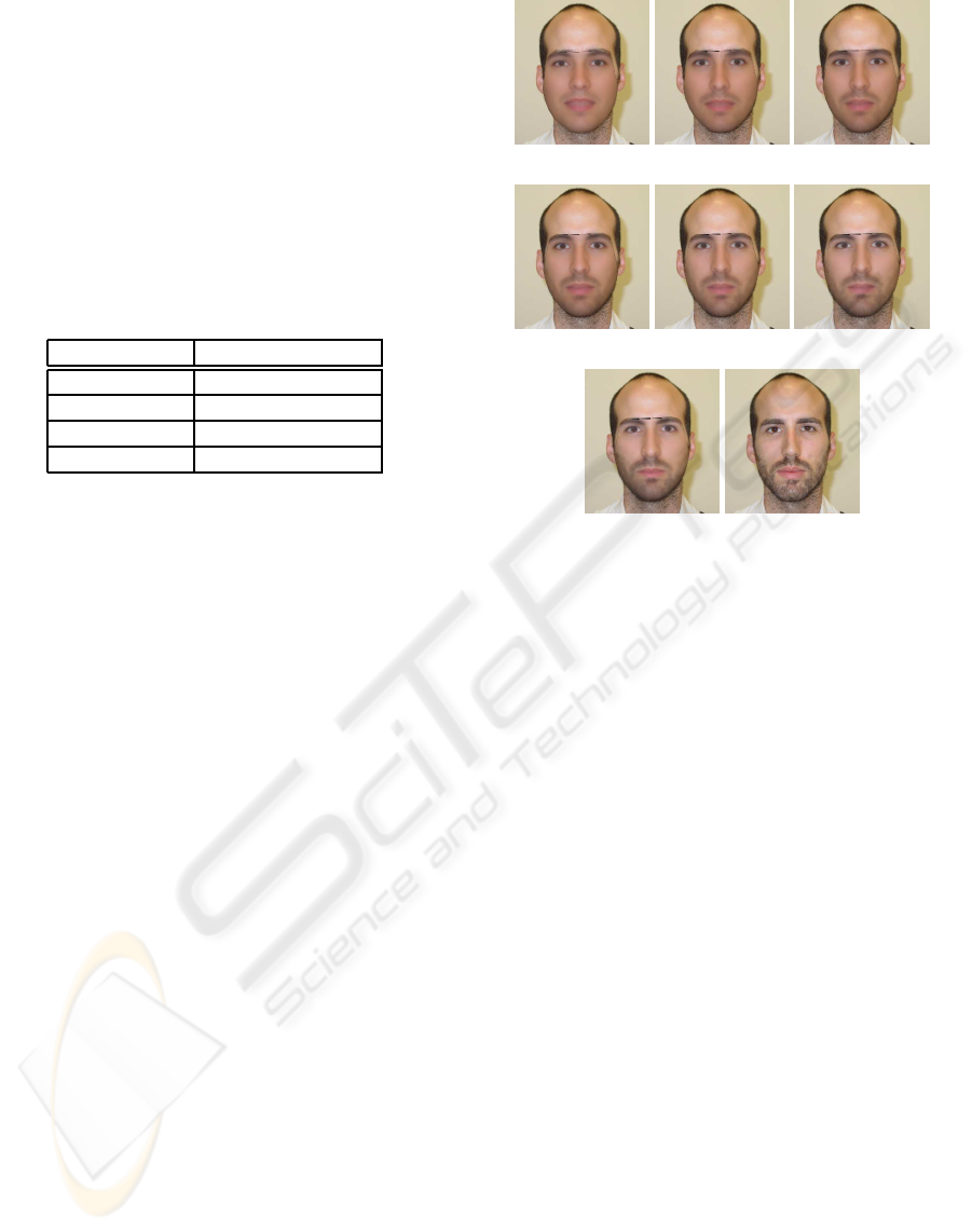
is made to error |δg|. Figure 3 shows a successful

AAM search. Note that, as better the initial estimate

is, minor the risk of being trap in a local minimum.

3 FACIAL EXPRESSION

RECOGNITION

3.1 Linear Discriminant Analysis

The facial expression recognition procedure is per-

formed by ﬁrstly describing a set of faces using

the AAM model (Bouchra Abboud, 2004). After-

wards, each vector of appearance c is projected into

(a) 1

(b) 2

(d) 4

(e) 5

(f) 6

(g) Final (h) Original

Figure 3: Iterative model reﬁnement.

Fisherspace, applying a Linear Discriminant Analy-

sis (LDA) (Peter N. Belhumeur and Kriegman, 1997).

This supervised learning technique consists in opti-

mizing the separability of the dataset observations ac-

cording to the expression class they belong to. This

is done by maximizing the between-class variance

while minimizing the within-class variance. These

variances are expressed by the two scatter matrixes

shown in eq. 18 and eq. 19.

∑

j=1

(µ

− µ)(µ

− µ)

(18)

∑

j=1

∑

i=1

− µ

)(X

− µ

)

(19)

In these expressions, n

is the number of classes,

represents the i

sample of class j, and µ

and µ

are the mean of class j and the mean of all classes,

respectively. This linear transformation of data will

allow subsequent classiﬁcation of new images repre-

senting one of the expression categories j.

3.2 LDA Evaluation Metric

Similary to a Principal Component Analysis, a LDA

transformation also involves performing an eigenvec-

tor decomposition which reﬂects the importance of

the data variance on the transformed subspace. The

VISAPP 2008 - International Conference on Computer Vision Theory and Applications

126

resulting data model retains the features that maxi-

mize class separability while holding a percentage of

the data variance.

In order to evaluate the quality of the data discrim-

ination, we developed a metric based on applying a k-

means clustering algorithm on the result of the LDA.

Let us consider the ideal case where all the observa-

tions were completely separated after LDA. In this

case, we could apply a clustering algorithm on the

data and obtain n

groups containing all faces with

the same expression. Table 2 shows what would be

the ideal clustering result for a dataset of n

subjects

per expression. Note that since there are seven ex-

pressions the k-means algorithm would be applied to

get seven groups.

Table 2: k-means clustering result for ideal LDA.

1 2 3 4 5 6 7

Neut n

0 0 0 0 0 0

Happ 0 n

0 0 0 0 0

Sad 0 0 n

0 0 0 0

Surp 0 0 0 n

0 0 0

Ang 0 0 0 0 n

0 0

Fear 0 0 0 0 0 n

Disg 0 0 0 0 0 0 n

The metric assigns a discrimination quality value

to the clustering result. Its value is calculated by sum-

ming the difference between the higher and the lower

values of each row of this table (i.e. the sum of the

degree of concentration of each class). The higher

the metric output, the better is the discrimination. By

applying this metric to several LDA runs, with differ-

ent number of features retained, we can estimate how

many modes of variation should be hold to optimize

the discrimination.

3.3 Classiﬁcation

Once deﬁned the axes that maximize the data classes

separability, it is possible to classify either training

images or unseen faces. The classiﬁcation for an un-

known face image consists in two steps. The ﬁrst is

projecting its appearance vector, c, on the hiperspace

that resulted from the trainning process. The second

is to estimate to each group does this projected point

belongs to. In our case this is done by using an adap-

tation of the nearest-neighbourhood algorithm, which

takes in consideration not only the distance of the

point to the centre of each group, but also its disper-

sion. The distance to each group is measured using

malahanobis distance (Krzanowski, 1988), eq. 20,

since it gives a scaled measure of an instance from

a particular class.

D = (c− c

)Σ

−1

(c− c

) (20)

is the vector of extracted appearance parame-

ters, c

is the centroid of the class multivariate distri-

bution and Σ is the within-class covariance matrix.

4 EXPERIMENTAL RESULTS

For the purpose of this work, an expression database

was built. It consists in 21 individuals showing 7

different facial expressions each. These expressions

are: neutral expression, happiness, sadness, surprise,

anger, fear and disgust. The data set is therefore

formed by a total of 147 colour images (640× 480).

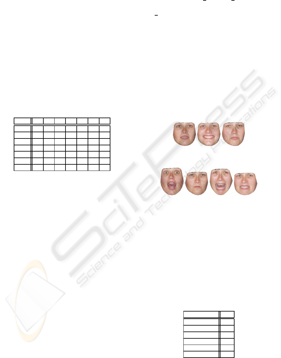
Figure 4 shows AAM model instances of a given sub-

ject for each one of the 7 facial expressions used.

(a)

Neutral

(b)

Happy

(d)

Surprise

(e) Anger (f) Fear (g)

Disgust

Figure 4: AAM instances of facial expressions used.

The AAM shape model was built using 58 anno-

tated landmarks (N = 58). The texture model was

generated sampling around 47000 pixels using also

colour information (g = 141000). Table 3 shows the

different values for retained variance used in each of

the three PCA that are required to create the combined

model, as well as the combined variation modes for

each one of this values.

Table 3: Retained variance and correspondent number of

modes, t

Variance(%) t

95.0 17

97.0 29

98.0 42

99.0 70

99.5 97

99.9 133

To evaluate the classiﬁcation results, a leave-one-

out cross-validation method was adopted. In this

FACIAL EXPRESSION RECOGNITION USING ACTIVE APPEARANCE MODELS

127

method each one of the dataset observations is used

once as the testing sample, while all the remaining

data is used for training.

4.1 First Experience - Optimizing AAM

and LDA variation Modes

In a ﬁrst experiment we studied the inﬂuence of the

variation modes retained either during AAM con-

struction or during LDA on the classiﬁcation perfor-

mance. On these experiment we used all the 147 im-

ages of the database. First we performed an evalua-

tion of the discrimination quality by varying the num-

ber of discrimination features retained on several face

models with different PCA variation modes retained.

As discrimination quality metric output depends on

the result of a k-means clustering, these tests were re-

peated for 250 times. A histogram of the best LDA

features retained in each trial was created for every

AAM model used. Figure 5 shows the result when

99.0% variation modes are retained on our dataset.

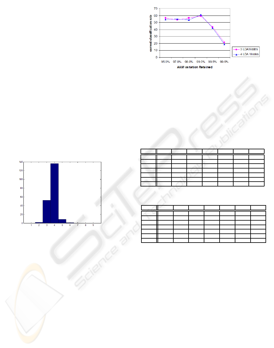
Figure 5: Histogram for best LDA modes on 250 trials.

As it can be seen, three or four LDA modes maxi-

mize the separation of classes. This was also observed

for 95.0% and 97.0% AAM variation modes.

Using these two values as LDA modes retained,

we performed leave-one-out cross-validation classi-

ﬁcation for face models with 95.0%, 97.0%, 98.0,

99.5% and 99.9% AAM modes. The global classi-

ﬁcation results are shown on ﬁgure 6.

It is clear from this graph observation that the clas-

siﬁcation performance varies with the percentage of

variation retained on the AAM construction process.

The best global classiﬁcations results were obtained

for 99.0% of variance retained.

4.2 Second Experiment - 7 Expressions

On the second experiment we analyse the classiﬁ-

cation performance for each expression. The same

dataset with 21 subjects in 7 different expressions is

Figure 6: Variation of global classiﬁcation results with dif-

ferent number of AAM modes retained.

used and a confusion matrix is created that represent

the classiﬁcation results for each expression. The re-

sults of the classiﬁcation for all datasets are resumed

on tables 4, 5 and 6 for different values of retained

variance.

Table 4: Confusion Matrix 97.0% Overal recognition rate = 55%.

Neut Happ Sad Surp Ang Fear Disg

Neut 19.0 0 52.38 0 9.52 19.05 0

Happ 0 90.48 0 0 0 4.77 4.77

Sad 9.52 0 61.90 4.77 9.52 14.29 0

Surp 0 0 0 80.95 0 19.05 0

Ang 0 0 14.29 0 33.33 9.52 42.86

Fear 0 4.77 9.52 19.05 14.29 52.38 0

Disg 0 14.29 0 0 38.10 0 47.62

Table 5: Confusion Matrix 98.0% Overal recognition rate = 56.5%.

Neut Happ Sad Surp Ang Fear Disg

Neut 33.33 0 61.90 0 0 4.76 0

Happ 0 80.95 0 0 0 9.52 9.52

Sad 0 4.76 66.67 0 19.05 9.52 0

Surp 0 0 0 71.43 0 28.57 0

Ang 0 4.76 4.76 0 42.86 14.29 33.33

Fear 0 4.76 9.52 19.05 9.52 52.38 4.76

Disg 0 9.52 0 0 38.10 4.76 47.62

We can see from this results that there is an ef-

fect of confusion between neutral and sad expres-

sions, and also between anger and disgust. This sug-

estes that there is an appearance correlation between

these two pairs of expressions. In fact, these results

are not surprising. Several neuroscience (Killgore and

Yurgelun-Todd, 2003) studies have showned that in

case of human emotion recognition, to percieve sad

and anger expressions, an especiﬁc cognitive process

is required.

4.3 Third Experiment - 5 Expressions

Experiment three tries to eliminate the confusion ef-

fect described on the previous experiment. Faces ex-

pressing sadness and anger were excluded both from

training and testing. The results of the classiﬁcation

for the same LDA and AAM conditions are expressed

on tables 7, 8 and 9.

VISAPP 2008 - International Conference on Computer Vision Theory and Applications

128

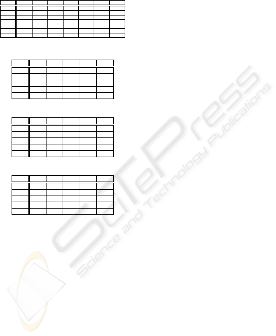
Table 6: Confusion Matrix 99.0% Overal recognition rate = 61.2%.

Neut Happ Sad Surp Ang Fear Disg

Neut 52.38 0 42.86 0 4.76 0 0

Happ 0 90.48 4.76 0 0 4.76 0

Sad 4.76 4.76 76.19 0 4.76 4.76 4.76

Surp 0 0 0 76.19 0 23.81 0

Ang 4.76 0 9.52 0 33.33 23.81 28.57

Fear 0 9.52 4.76 14.29 4.76 66.67 0

Disg 0 23.81 4.76 0 33.33 4.76 33.33

Table 7: Confusion Matrix 97.0% Overal recognition rate = 74.3%.

Neut Happ Surp Fear Disg

Neut 57.14 0 0 42.86 0

Happ 0 90.48 0 9.52 0

Surp 0 0 76.19 23.81 0

Fear 9.52 4.76 23.81 61.90 0

Disg 0 9.52 0 4.76 85.71

Table 8: Confusion Matrix 98.0% Overal recognition rate = 76.2%.

Neut Happ Surp Fear Disg

Neut 90.48 0 0 9.52 0

Happ 0 85.71 0 4.76 9.52

Surp 0 0 71.43 28.57 0

Fear 4.76 4.76 19.05 66.67 4.76

Disg 0 19.05 0 14.29 66.67

Table 9: Confusion Matrix 99.0% Overal recognition rate = 63.8%.

Neut Happ Surp Fear Disg

Neut 80.95 9.52 4.76 4.76 0

Happ 9.52 66.67 0 14.29 9.52

Surp 4.76 0 66.67 28.57 0

Fear 4.76 9.52 28.57 52.38 4.76

Disg 9.52 23.81 4.76 9.52 52.38

5 CONCLUSIONS

We used standart AAM model to discribe face entities

in a compact way. With LDA we are able to separate

the several emotion expression classes and perform

classiﬁcation using mahalanobis distance.

On the AAM model building process, holding

more information on the appearance vectors not al-

ways results on a better discrimination result. In our

experiments, this value rounds 99.0% of variance re-

tained.

The number of LDA eigenvectors used is another

parameter of great importance. K-means is used in

order to give us a good estimation for this value.

As expected, the larger the number of expressions

used, the worse is the overal successful classiﬁcation

rate. The reason for this is that there are correlations

between the two pairs of expressions neutral, sad and

anger, disgust, comproved by psico-physics studies.

We achieved, with all the seven expressions, an

overal successful recognition rate of 61.1%. Remov-

ing correlated expressions, this recognition rate in-

creases to a maximum of 76.2%.

REFERENCES

Batista, J. P. (2007). Locating facial features using an an-

thropometric face model for determining the gaze of.

faces in image sequences. ICIAR2007 - Image Analy-

sis and Recognition.

Bouchra Abboud, Frank Davoine, M. D. (2004). Facial

expression recognition and synthesis based on an ap-

pearance model. Signal Processing Image Communi-

cation.

G. Finlayson, S. Hordley, G. S. and Tian, G. Y. (2005). Il-

luminant and device invariant color using histogram

equalisation. Pattern Recognition.

Killgore, W. D. and Yurgelun-Todd, D. A. (2003). Acti-

vation of the amygdala and anterior cingulate during

nonconscious processing of sad versus happy faces.

NeuraImage.

Krzanowski, W. J. (1988). Principles of multivariate analy-

sis. Oxford University Press.

Peter N. Belhumeur, J. P. H. and Kriegman, D. J. (1997).

Eigenfaces vs. ﬁsherfaces: Recognition using class

speciﬁc linear projection. IEEE Transactions on Pat-

tern Analysis and Machine Intelligence.

P.Viola and Jones, M. (2004). Rapid object detection using

a boosted cascate of simple features. Proceeding of

the IEEE Conference on Computer Vision and Pattern

Recognition.

Stegmann, M. B. (2000). Active appearance models theory,

extensions & cases. Master’s thesis, IMM Technical

Univesity of Denmark.

Stegmann, M. B. and Gomez, D. D. (2002). A brief intro-

duction to statistical shape analysis. Technical report,

Informatics and Mathematical Modelling, Technical

Univesity of Denmark.

T. Dalgleish, M. P. (1999). Handbook of cognition and emo-

tion. John Wiley & Sons Ltd.

T.F.Cootes and C.J.Taylor (2004). Statistical models of ap-

pearance for computer vision. Technical report, Imag-

ing Science and Biomedical Engineering - University

of Manchester.

T.F.Cootes, G. E. and C.J.Taylor (2001). Active appearance

models. IEEE Transactions on Pattern Analysis and

Machine Intelligence.

FACIAL EXPRESSION RECOGNITION USING ACTIVE APPEARANCE MODELS

129