
AN ONLINE SELF-BALANCING BINARY SEARCH TREE FOR
HIERARCHICAL SHAPE MATCHING
N. Tsapanos, A. Tefas and I. Pitas
Department of Informatics, University of Thessaloniki, Box 451, 54124 Thessaloniki, Greece
Keywords:
Hausdorff Distance, Hierarchical Shape Matching, Binary Search Trees.
Abstract:
In this paper we propose a self-balanced binary search tree data structure for shape matching. This was
originally developed as a fast method of silhouette matching in videos recorded from IR cameras by firemen
during rescue operations. We introduce a similarity measure with which we can make decisions on how to
traverse the tree and backtrack to find more possible matches. Then we describe every basic operation a binary
search tree can perform adapted to a tree of shapes. Note that as a binary search tree, all operations can be
performed in O(logn) time and are very fast and efficient. Finally we present experimental data evaluating the
performance of our proposed data structure.
1 INTRODUCTION
Object recognition by shape matching traditionally
involves comparing an input shape with various
templates and reporting the template with the high-
est similarity to the input shape. As the template
database becomes larger, exhaustive search becomes
impractical and the need of a better way to organize
the database aiming to optimize the cost of the search
operations arises.
Recently, Gavrila proposed a bottom-up tree
construction based on grouping similar shapes
together in size-limited groups, then selecting a
representative of the group and repeating, until a tree
similar to B-trees is formed (Gavrila, 2007). While
searching, the traversal of more than one children of
any node is permitted. However, this structure does
not provide any worst case performance guarantee
and no way to add further shapes without having to
reconstruct the tree.
Self-balancing binary search trees are well
known data structures for quick search, insertion and
deletion of data. In this paper we propose a way to
adapt this kind of data structure to a tree of shapes.
By doing so we can search, insert and delete shapes
Research was supported by the project SHARE: Mo-
bile Support for Rescue Forces, Integrating Multiple Modes
of Interaction, EU FP6 Information Society Technologies,
Contract Number FP6-004218.
in logarithmic worst case time.
The main issue we have to address is that
shape similarity is much less strict than number
ordering (for example, shape dissimilarity is not
transitive). This means that in order for a node to
make a decision on which child to direct a search that
node must have a more complicated decision criterion
and undergo training for that criterion. The training
must also be independent of the number of nodes in
the tree. Conversely, we provide no guarantee that
the best match will be found. However, experimental
data indicate that, given enough tries to backtrack,
our trees can learn the training set almost perfectly.
For our purposes, we view a shape as a set
of points with 2-dimensional integer coordinates.
Sets of points are referred to by capital letters and a
single point of a set by the same letter in lowercase.
Shapes from the training set and those produced by
our algorithms at various points are referred to as
templates.
This paper is organized as follows: section
2 briefly introduces the similarity measure that we
use to traverse our tree, section 3 explains the types of
tree nodes and their contents, section 4 describes all
the basic tree operations (search, insertion, deletion,
rotations), section 5 presents experimental data and
section 6 concludes the paper.
591
Tsapanos N., Tefas A. and Pitas I. (2008).
AN ONLINE SELF-BALANCING BINARY SEARCH TREE FOR HIERARCHICAL SHAPE MATCHING.
In Proceedings of the Third International Conference on Computer Vision Theory and Applications, pages 591-597
Copyright
c
SciTePress
2 SIMILARITY MEASURE
The similarity measure of our choice is based on the
Modified Hausdorff Distance (MHD):
D
MHD
(X,T) =
1
|X|
∑
x∈X
d(x,T) (1)
We introduce an activation function through which
the individual distances d(x,T) = min
t∈T
||x−t||
2
are
passed before the sum. We call this similarity mea-
sure the Activated Hausdorff Proximity (AHP)
sim(X,T) = P
AHP
(X,T) =
1
|X|
∑
x∈X
e
−αd(x,T)
(2)
where X is the test set of points, T is the set of points
forming a template with which X is matched and α is
a constant.
We use this activation function in order to normal-
ize the similarity measure to (0, 1], 1 meaning that
there is a point in T exactly on every point in X and,
as dissimilarity increases, our measure tends to 0.
In practice we use a distance transform on the tem-
plate T that outputs a matrix {a
ij
} such that each el-
ement a
ij
is the integer approximation of the distance
of point x with coordinates (i, j) from the closest point
in T a
ij
≈ d(x,T). We then use a precomputed array
with the values of e
−αk
for every integer k that we
expect from the distance transform. This way, for ev-
ery point x we can find e
−αd(x,T)
with only 3 memory
references.
3 TREE NODES
There are two types of nodes in our binary search tree:
template nodes and internal nodes.
3.1 Template Nodes
A template node contains a single real template from
the training set. The template is stored as a set of
2-dimensional points with integer coordinates. The
distance transform of the template is stored here as
well. Template nodes can only be leaf nodes.
3.2 Internal Nodes
The internal nodes are dummy nodes. They do not
contain any real information and they are used to de-
termine the search path to the leaf nodes where the
actual data is stored. They cannot be leaf nodes them-
selves.
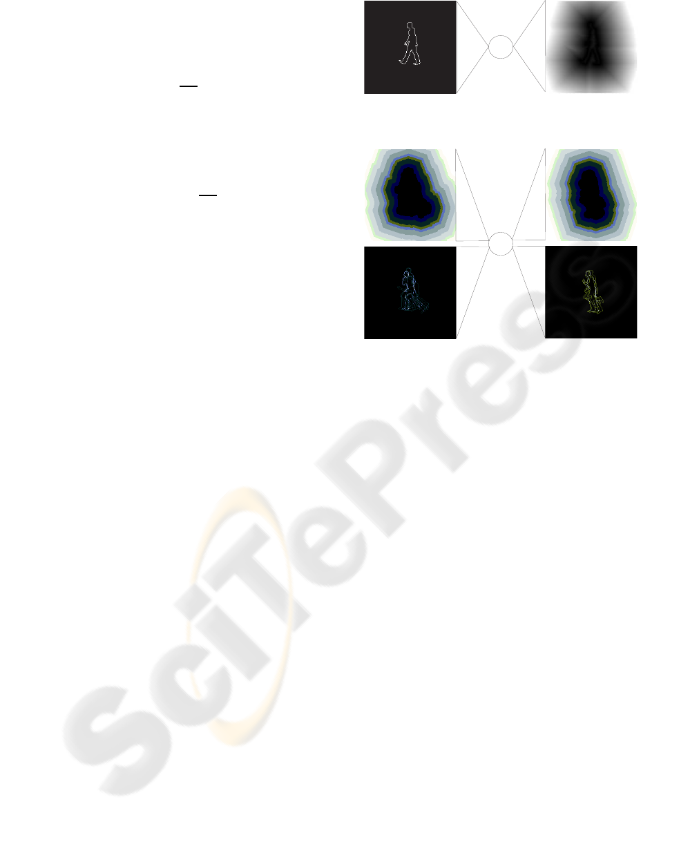
Figure 1: A template node.
Figure 2: An internal node.
Each internal node contains the distance transform
of a ”left” template T
L
and the distance transform of
a ”right” template T
R
, a matrix with the sum of every
real template that is under it’s left subtree S
L
, another
matrix with the sum of every real template under it’s
right subtree S
R
and also other information regard-
ing the structure and balance of the tree (pointers to
other nodes, node balance for AVL trees, colour for
red/black trees etc).
The decision on which path to follow for a test
set of points X is made by calculating sim(X,T
L
)
and sim(X,T
R
) and then directing the search to the
subtree that produces the largest value in our sim-
ilarity measure. Thus, an internal node directs the
search to it’s left subtree, if sim(X, T
L
) > sim(X,T
R
),
or the right subtree otherwise, with confidence c =
|sim(X,T
L
) −sim(X,T
R
)|. This confidence measure
will later help us backtrack the search in order to find
better results we may have missed.
4 ONLINE TREE
Online trees are created by incrementally inserting ev-
ery template of the training set. In this section we will
describe how all the tree operations are performed.

4.1 Search
We will now describe how to find the closest match
of a set of points X in our tree. Starting from the root
of the tree we follow the path of nodes as dictated by
comparing the similarities of X with each node’s T
L
and T
R
until we reach a leaf. Then we report the tem-
plate of that leaf as a possible result. Since we replace
the constant time operations of a binary search tree
with operations that also require constant time (with
respect to the number of nodes n), this can be done in
O(logn) time as per the binary search tree bibliogra-
phy.
Due to the non-strict nature of the Hausdorff dis-
tance and therefore our similarity measure too, we
cannot give any guarantees that the first result of a
search is the best one. To overcome this we note the
confidence of each node in the path to the previous
result and we backtrack through the path and reverse
the decision of the node with the lowest confidence
and proceed to search the subtree we skipped in the
previous search. Once a nodes decision has been re-
versed, we set it’s confidence to 1, so that it won’t
switch again until the search is over.
This way, if we allow r tries, we come up with r
template candidates. We determine the best match
by exhaustive search between these candidates. This
takes us O(rlogn) time to do.
Regarding the values of nodes’ confidence along
the path to a leaf, what we expect is that the confi-
dence will be lower toward the end of the path (be-
cause the templates with a low least common ances-
tor will be similar) and toward the root of the path
(because there will be a lot of templates to separate in
each subtree). It would be a good idea to replace the
confidence by a function of |sim(X,T
L
) −sim(X,T
R
)|
and the depth of a node, however we find that it is
more practical to artificially restrict switching paths
at the higher levels in the first few tries.
4.2 Insertion
To insert a new node q
n+1
with a template T
n+1
into
the tree we start by searching for T
n+1
in the current
tree. If we come to an internal node with only 1 child
during our search, we add the new node as it’s other
child. If the search stops at a leaf node q
i
, we replace
it with an internal node and add q
n+1
and q
i
as the new
internal node’s children. The template T
n+1
is also
added to the proper sum matrix (S
L
or S
R
) of every
node it traverses.
This means that the new template will be inserted
near similar templates and guarantees that if we
search for the template again, the search will find it
in the first try (provided no tree rotations have been
performed since it’s insertion).
After inserting a node, we then follow the reverse
path to the root, balancing and retraining every af-
fected node. Again, the changes we propose involve
constant time operations (node training is indepe-
dent from the number of nodes n), so insertion takes
O(logn) time as a property of binary search trees.
4.3 Deletion
Our tree only supports the deletion of leaf nodes.
Moreover, we feel that the task of deleting a node
based on an input shape is not well defined. Trying
to delete a template we have not yet stored by search-
ing for it first will result in the deletion of the template
that is the closest match for it, something that is prob-
ably not what we wanted. Even if the template exists
in the tree, the search operation is not guaranteed to
find it.
In this section we will describe the deletion of a
leaf whose location must be known beforehand. De-
termining which leaf we want to delete is subject to
the deletion policy we wish to enforce (and using ad-
ditional data structures). For example, if we want to
delete the oldest template at a time we can maintain a
queue of pointers to the templates in the order they are
inserted into the tree. If we want to delete nodes on
a least recently used basis, we will probably need to
maintain a minimum-heap data structure for the use
of the nodes. While there is nothing preventing the
deletion of a search result, we must note that doing so
is unadvisable.
Starting from the node q
j
which want to delete, we
travel backwards to the root via parent node pointers.
The reverse path is what we need to proceed with the
deletion as per normal binary search trees. We sub-
tract the nodes template T
j
from the proper sum (S
L
or
S
R
) of each node traversed and rebalance where nec-
essary.
Deleting nodes and rebalancing can result in an in-
ternal node with no children. Since we do not allow
that, we check whether an internal node is left child-
less, mark that node for deletion and repeat the pro-
cess again.
n1
S
rl
n3
S
rr
n2
s2
s3
s4
s1
S
ll
S
lr
n1
S
rl
S
rr
n3
S
lr
n2
s3
s4
s2
s1
S
ll
S+
ll
S
lr
S+
rl
S
rr
n2
S
ll
S
rl
n1
S
rl
S
rr
n3
s1
s2 s3
s4
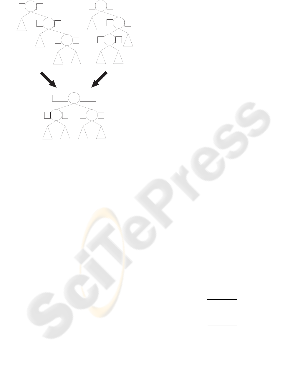
Figure 3: After proper assignment of the nodes and matri-
ces, the steps to perform the rotation are predetermined.
4.4 Balancing
The tree can be of any type of self-balancing tree that
achieves balance by using tree rotations. In our im-
plementation it’s an AVL-tree (Adelson-Velskii and
Landis, 1962).Here we will describe the LL and RL
rotations (the RR and LR cases are symmetrical).
To simplify the description and the implementation,
we name the three nodes involved in the rotation
n
1
,n
2
,n
3
, the subtrees from left to right s
1
,s
2
,s
3
,s
4
and the sum of each subtree S
ll
,S
lr
,S
rl
,S
rr
. See figure
3 for details.
After the rotation:
• n
2
is the parent of n
1
and n
3
with S
(n
2
)
L
= S
ll
+ S
lr
and S
(n
2
)
R
= S
rl
+ S
rr
• n
1
is the left child of n
2
with S
(n
1
)
L
= S
ll
and S
(n
1
)
R
=
S
lr
• n
3
is the right child of n
2
with S
(n
3
)
L
= S
rl
and
S
(n
3
)
R
= S
rr
Every rotation can be performed by properly as-
signing n
1
, n
2
, n
3
, s
1
, s
2
, s
3
, s
4
, S
ll
, S
lr
, S
rl
, S
rr
and
performing a set reconnection.
4.4.1 Ll Rotation
This is a very straight forward case. See Figure 3.
4.4.2 RL Rotation
After an RL (or LR) rotation in a normal binary search
tree, a leaf maybe become an internal node and vice
versa. In our tree, template nodes cannot be internal
nodes and internal nodes cannot be leaf nodes. In our
tree, however, the ordering of the nodes is not strictly
numeric, so we can slightly alter the rotation to satisfy
our restrictions. See Figure 3.
4.5 Node Training
The object of node training is to find the templates
T
L
and T
R
such that would, ideally, direct every leaf
node template to the correct subtree. Unfortunately,
we have no way of guaranteeing this without exceed-
ing logarithmic time. We try to approximate the tem-
plates T
L
and T
R
using two methods.
4.5.1 Fast Method
The fastest method is to simply extract the template
T
L
from S
L
and T
R
from S
R
. S
L
is the sum of every
template in the left subtree, so we can scan the ma-
trix to find all the non-zero entries and build the set
of points for T
L
from the matrix coordinates of those
entries (likewise for T
R
).
4.5.2 Abstractive Method
Instead of select every point from S
L
and S
R
, we can
focus on selecting the points that differentiate the ma-
trices S
L
and S
R
. We do this by computing a weighted
centroidal voronoi tesselation (CVT) simplification
(A. Hajdu and Pitas, 2007) of each set of points.
Let L be the set of points extracted from S
L
and R
be the set of points extracted from S
R
. For every point
l ∈ L we set the weight
ρ(l) =
1
1+ e
−αd(l,R)
(3)
and for every point r ∈ R
ρ(r) =
1
1+ e
−αd(r,L)
(4)
Note that the units in equation (3) are in fact e
−αd(l,L)
butsince l ∈L, d(l,L) = 0 (likewisefor equation (4) ).
Then we iteratively compute the CVT simplifi-
cation of L and R to obtain T
L
and T
R
. Using the
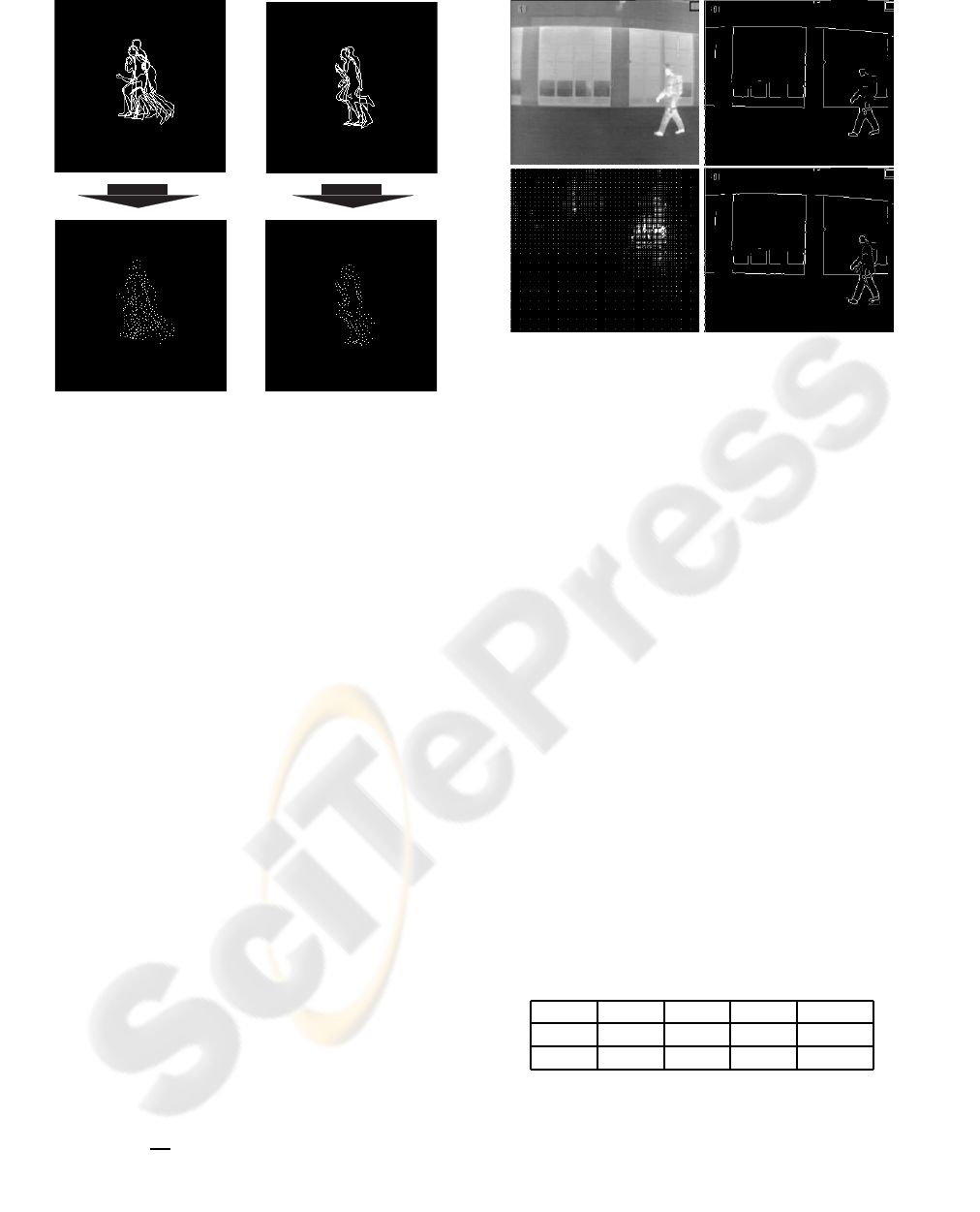
Figure 4: T
L
and T
R
as extracted from S
L
and S
R
and after
their CVT simplification.
above weight functions, the simplification algorithm
for L is less likely to select points closer to R
favouring points that are further away from it (and
vice versa). The results of a CVT simplification can
be seen in fig. 4.
5 EXPERIMENTS
We tested our tree in the task of matching silhouettes
of humans in thermal videos available from a fire de-
partment for the purposes of rescue operations. In or-
der to search for a template in our tree in an image
we proceed as follows: First, we perform edge detec-
tion on the image, then search in the edgemap. At any
point in the edgemap we find the relative coordinates
of every edge in the search window. Then we try to
find the best matching template for these points in our
tree (we find T
best
= argmin
T
(P
AHP
(X,T))) then we
compute the reverse proximity of that template to the
edgemap (P
AHP
(T
best
,X)). We report the point and
template with the best overall reverse proximity.
Scale is addressed simply by adding the scaled tem-
plates into the same tree with the original templates.
The spatial search in the edge map is pruned by scan-
ning the image with a step of s = 16 and recursively
reducing the step by 1/2 if the reverse proximity ex-
ceeds a threshold. This threshold is determined by the
function e
−α
√
2s
2
. The constant α is set to 0.1. Rota-
tion is not addressed, but we can handle it either by
inserting rotated templates into the tree, or searching
Figure 5: The original image, it’s edgemap, the pruned
search space and the final result.
in rotated images (again pruning the search space us-
ing thresholds). Figure 5 shows some of the stages of
the process and figure 6 shows the output of our tree
for a few frames.
5.1 Learning Capabilities
We first tried to determine whether our tree is capable
of learning the training set of templates and how many
tries does it take so that the search for every template
returns the exact template it was searching for.
Starting with a set of 43 human silhouettes, we con-
structed a training set for the tree that includes the
43 original templates, the templates scaled down by
10%, scaled up by 10%, 20%, 30% and 40% and the
mirror image of all the scaled templates. This resulted
in 516 templates that we inserted into an empty start-
ing tree. Below is a table with the number of cor-
rect answers and average time per search of our tree
with 1,2,4,8 tries and the time of the exhaustive search
(time in milliseconds).
Table 1: Tree learning capabilities.
1 2 4 8 Ex
500 504 516 516 516
0.081 0.165 0.295 0.512 3.0935
As evident, with as little as 4 tries to backtrack, our
tree can learn the 516 templates of our training set. In
our further experiments, the tries are set to 8 because
we will be dealing with real data. Note that even with
8 tries, our tree takes about 1/6 of the time the exhaus-
tive search needs.
5.2 Comparison with Exhaustive
Template Searching
We now compare the performance of our tree against
exhaustive search in 4 scenes of thermal video (all
scenes were 321 by 278 pixels). We measure time and
the difference in reverse proximity of both methods of
searching. The spatial search is pruned for both meth-
ods and the time for edge detection is not included.
Measurements are presented as mean (standard de-
viation) and measure the average time per search in
milliseconds and the difference in reverse proximity.
Table 2: Tree and exhaustive search results.
Scene 1 Scene 2
Frames 1176 426
Ex. time 7020(7906) 4851(3393)
Tr. time 757(872) 525(328)
Pr. diff -0.033(0.039) -0.033(0.034)
Scene 3 Scene 4
Frames 1026 226
Ex. time 13199(9187) 12076(10656)
Tr. time 1318(969) 1247(1113)
Pr. diff -0.044(0.039) -0.046(0.038)
Our tree takes about 1/10 of the time the exhaustive
search takes and the difference in the reverse proxim-
ity of the answers is minimal. Also note that on some
occasions our tree finds an answer with a larger re-
verse proximity than the exhaustive search.
5.3 Comparison with Fully Exhaustive
Searching
Finally, we measure the overall gain in time and
loss in quality between our tree in a pruned search
space and the fully exhaustive search (measures re-
verse proximity for every template at every location)
in a scene with 117 frames.
Table 3: Comparison with fully exhaustive search.
Full ex. time Tree time Prox. diff
305092(51134) 850(270) -0.039(0.037)
Compared to the fully exhaustive search, the tree
only takes 0.2% of the time, while the drop in quality
remains at the same negligible levels.
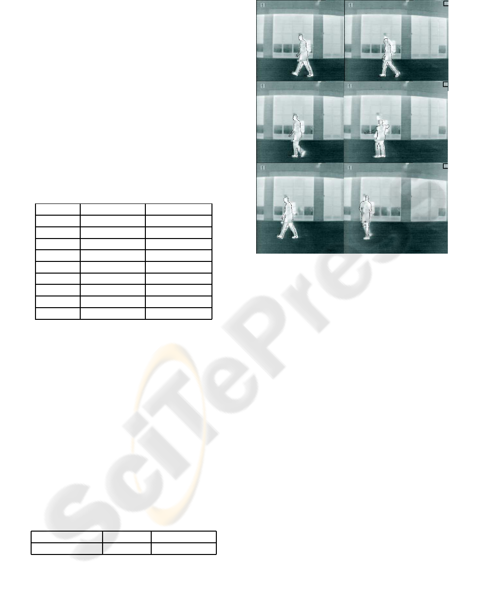
Figure 6: A few (non consecutive) frames showing the out-
put of our tree.
6 CONCLUSIONS
In this paper, we have described the basic operations
that a binary tree need to function, so that we can
quickly store and retrieve shapes instead of numbers
in a very fast and efficient data structure. Insertion
does not require the complete or even partial recon-
struction of the tree. Using the fast training method,
insertion takes about the same time as a single search.
Early tests indicate that the quality of results
that our proposed data structure produces is very
close to those that an exhaustive search would pro-
vide. The strengths of a binary search tree, however,
lie in the it’s speed and the ability to dynamically
insert new nodes efficiently.
Now that we have found a way to traverse a bi-
nary search tree of shapes (with a couple of templates
and AHP) and seeing that such a data structure can
work just as well as exhaustively searching, we can
further study the possibility of training a tree offline.
We can take advantage of the ample training time to
guarantee that each template will end up on the node
that contains it on the first try.
We can then study the generalization abilities of
the offline constructed trees and set a smaller number

of allowed tries for even faster searching and better
results. We can always add new nodes to an offline
constructed tree just like an online tree, if we need to.
REFERENCES
A. Hajdu, C. G. and Pitas, I. (July 2007). Object simplifica-
tion using a skeleton-based weight function. In Inter-
national Symposium on Signals, Circuits and Systems,
Volume 2, pp. 1-4.
Adelson-Velskii, G. M. and Landis, E. M. (1962). An algo-
rithm for the organization of information. In Doklady
Akademii Nauk SSSR, Volume 146, pp. 263-266.
Borgefors, G. (June 1986). Distance transformations in dig-
ital images. In Computer Vision, Graphics, and Image
Processing, Volume 34 , Issue 3, pp. 344-371.
Borgefors, G. (Nov. 1988). Hierarchical chamfer matching:
a parametric edge matching algorithm. In IEEE Trans-
actions on Pattern Analysis and Machine Intelligence,
Volume 10, Issue 6, pp. 849-865.
D. Huttenlocher, G. K. and Rucklidge, W. (Sep. 1993).
Comparing images using the hausdorff distance. In
IEEE Trans. Pattern Analysis and Machine Intelli-
gence, vol. 15, no. 9, pp. 850-863.
Gavrila, D. M. (Aug. 2007). A bayesian, exemplar-based
approach to hierarchical shape matching. In IEEE
Transactions on Pattern Analysis and Machine Intel-
ligence, Volume 29, Issue 8, pp. 1408-1421.
L. Ju, Q. D. and Gunzburger, M. (Oct. 2002). Probabilistic
methods for centroidal voronoi tessellations and their
parallel implementations. In Parallel Computing, Vol-
ume 28 , Issue 10, pp. 1477-1500.
Q. Du, V. F. and Gunzburger, M. (Dec. 1999). Centroidal
voronoi tessellations: Applications and algorithms. In
SIAM Review archive Volume 41, Issue 4, pp. 637-676.
Rucklidge, W. (June 1995). Locating objects using the
hausdorff distance. In Proceedings of Fifth Interna-
tional Conference on Computer Vision, pp. 457-464.
S. Belongie, J. M. and Puzicha, J. (Apr. 2002). Shape
matching and object recognition using shape contexts.
In IEEE Transactions on Pattern Analysis and Ma-
chine Intelligence Volume 24 , Issue 4, pp. 509 - 522.
