THE GROUNDED HEIGHTMAP TREE

A New Data Structure for Terrain Representation

J. Alonso and R. Joan-Arinyo

Grup d’Inform`atica a l’Enginyeria

Escola T`ecnica Superior d’Enginyeria Industrial de Barcelona

Universitat Polit`ecnica de Catalunya, Av Diagonal 647, 8

, 08028 Barcelona, Spain

Keywords:

Digital terrain model, Terrain modelling, Heightmaps.

Abstract: Terrain modeling is a fast growing ﬁeld with many applications such as computer graphics, resource man-

agement, Earth and environmental sciences, civil and military engineering, surveying and photogrammetry

and games programming. One of the most widely used terrain model is the Digital Elevation Model (DEM).

A DEM is a simple regularly spaced grid of elevation points that represent the continuous variation of relief

over space. DEMs require simple storage and are compatible with satellite data. However, they do not easily

account for overhangs.

In this work we report on the Grounded Heightmap Tree, a new data structure for terrain representation built

as a generalization of the DEM. The new data structure allows to naturally represent terrain overhangs. We

illustrate the performance of the Grounded Heightmap Tree when applied to represent terrains that undergo

big changes.

1 INTRODUCTION

Terrain modeling is a fast growing ﬁeld with many ap-

plications such as computer graphics, resource man-

agement, Earth and environmental sciences, civil and

military engineering, surveying and photogrammetry

and games programming. Since, in general, terrain

models store huge amount of data, and applications

must be highly responsive, having a model that al-

lows quick answers to the queries on it would be para-

mount.

One of the terrain models most widely used is

the Digital Elevation Model (DEM), also known as

heightmap, that requires simple storage, is compatible

with satellite data and allows good and simple surface

analysis. On the other hand, they are slow to compute

and are severely limited by the need of the uniform

sampling and do not easily account for overhangs.

This work reports on the development of a new data

structure, called Grounded Heightmap Tree, to model

and deal with terrains that change at a high rate to

capture, for example, big changes resulting from geo-

tectonic events. It is a generalization of the heightmap

model and accounts for hangovers.

2 TERRAIN MODELS

Basically, terrain models belong to one one of three

categories: Digital Elevation Models (DEM), Trian-

gulated Irregular Networks (TIN) and Fractal Mod-

els. DEMs have been applied to represent terrains

over uniformly distributed sample points. TINs allow

representing real terrains with a high ﬁdelity over ir-

regular networks of sample points. Fractal Models are

used to represent terrain models randomly generated.

2.1 Digital Elevation Model

DEMs are based on a simple structure named

heightmap also known as heightﬁeld. A heightmap

is simply a 2D array of values which give the terrain

elevations for ground positions sampled at regularly

spaced horizontal intervals. Each value in the array

represents the height of the terrain at that value’s po-

sition. See Figure 1, (Robot-frog, ). For example, if

the cell at (2, 3) has a value of 2, then the terrain con-

tains the point (2, 3, 2).

On the one hand, DEMs require simple storage,

are compatible with satellite data and allow good and

simple surface analysis. On the other, they are slow

to compute and are severely limited by the need of

the uniform sampling and do not easily account for

Alonso J. and Joan-Arinyo R. (2008).

THE GROUNDED HEIGHTMAP TREE - A New Data Structure for Terrain Representation.

In Proceedings of the Third International Conference on Computer Graphics Theory and Applications, pages 80-85

DOI: 10.5220/0001094300800085

 SciTePress

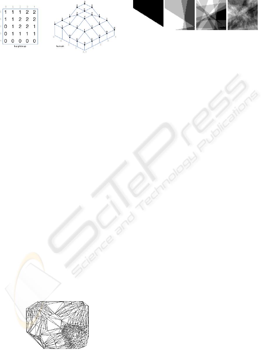
Figure 1: Digital Elevation Model. Left) Heightmap. Right)

3D terrain wireframe.

overhangs.

2.2 Triangulated Irregular Networks

A TIN is a DEM with a network of non-overlapping

triangles whose vertices are placed at randomly lo-

cated terrain points. These triangles are formed usu-

ally under Delaunay criterion. Irregular spaced sam-

ple points are measured with more points in areas of

rough terrain and fewer in smooth terrain which re-

sults in an accurate representation of the terrain. Fig-

ure 2 shows a TIN, (Klinkenberg, ).

Pros of the TINS are that they need fewer points

than DEMs for the same accuracy, their resolution

naturally adapts to terrain roughness. Among the

drawbacks we ﬁnd that initial construction is time

consuming and some operations do not have efﬁcient

algorithms.

2.3 Fractal Models

Historically, fractals have been one of the pioneering

technique representation chosen by terrain rendering

and visualization researchers. Examples of methods

to generate fractal terrain models are diamond-square

algorithm, fault algorithm and the hill algorithm.

These techniques take as input a 2D array whose cells

are properly initialized, and iteratively transform it

until a ﬁnal terrain representation is reached.

The diamond-square algorithm is a method for

generating highly realistic heightmaps for computer

Figure 2: Triangulated Irregular Network.

Figure 3: Fault formation. Terrain height map evolution as

the number of iterations increases.

graphics, (Martz, ). The starting point for the itera-

tive technique sets the four corner points of an array

to the same height value. Notice that what we have

got is a square. Then there are two different possi-

ble steps: the diamond step or the square step. The

diamond step takes a square and generates a random

value at the square midpoint, where the two diagonals

meet. The midpoint value is calculated by averaging

the four corner values, plus a random amount. This

gives us diamonds when we have multiple squares

arranged in a grid. The square step takes a diamond

and generates a random value at the center of the dia-

mond. The midpoint value is calculated by averaging

the corner values, plus a random amount generated in

the same range as used for the diamond step. This

gives us squares again. Now the algorithm iterates

performing one diamond step, one square step and a

reduction of the random values range until the length

of the squares side is smaller than a given threshold.

Fault formation is a very simple one, yet its re-

sults, although not the best, are pretty good, (Fault

algorithm, ). The technique is not limited to pla-

nar height ﬁelds, being also applicable to spheres to

generate artiﬁcial planets. Hugo Elias (Elias, ), has

posted tutorials on the application of this algorithm to

spheres. To start with we have a planar height ﬁeld,

where all points have zero height. Then we select

a random line which divides the terrain in two parts

(in general these parts will be different in size). The

points to one side of the line will have their height

displaced upwards, whereas the points on the other

side will have their heights displaced downwards. So

now we have a terrain with two distinct heights. If

we keep dividing the terrain like this then we will get

something that has valleys, mountains and so on. Fig-

ure 3 illustrates the process where the 2D array is re-

cursively split.

The hill technique can be seen as a kind of fault

formation where the straight line used to divide the

terrain is replaced with an sphere. The basic idea is

simple, (Robot-frog, ). Start with a ﬂat terrain (ini-

tialize all height values to zero). Pick a random point

on or near the terrain, and a random radius between

some predetermined minimum and maximum. Care-

fully choosing these values will make a terrain rough

and rocky or smooth and rolling. Raise a hill on the

THE GROUNDED HEIGHTMAP TREE - A New Data Structure for Terrain Representation

Figure 4: Left: Isolated hill. Right: The model after several

iterations.

terrain centered at the point, having the given radius.

Repeat the two previous steps as many times as neces-

sary. Notice that the number of iterations chosen will

affect the appearance of the terrain. Figure 4 depicts

on the left an isolated hill and on the right the model

after performing several iterations.

3 THE GHT MODEL

As presented in Section 2, heightmaps offer a good

balance between complexity and performance. How-

ever, this balance is broken when trying to capture

terrains with overhangs. The GHT model presented

in this work is a generalization of the heightmaps that

easily accounts for both overhangs and tunnels while

basically keeping the simplicity of heightmaps. It is

specially well suited to capture terrains built through

a sculpting process from an initial 2D grid of terrain

elevations.

3.1 Deﬁnitions

The model deﬁnition is rather simple. The grounded

heightmap tree is a tree where the nodes are grounded

heightmaps and the edges are pointers to other

grounded heightmaps.

A grounded heightmap is a ground plane along

with an axis aligned 2D array of data cells. The

ground plane is deﬁned by a point and the direction

vector. Each data cell contains a height measured

with respect to the ground plane along its direction

vector, and a pointer to some data cell in a different

grounded heightmap. To properly manage carvings

and hangovers, the GHT model includes the

type

tag

which distinguishes whether a grounded heightmap is

an outdoor area, is an indoor area (carving or hang-

over) or is a heightmap which deﬁnes the transition

between indoor and outdoor areas. Figure 5 shows

the GHT data type deﬁnition using C-like notation.

3.2 Model Construction

Constructing a GHT model starts with just one

grounded heightmap whose ground plane is the XZ

typedef struct{

DataArray data;

GroundPlane gplane;

GroundedHeightmap *child;

TerrainType type;

} GroundedHeightmap;

typedef DataArray DataCell [1..N][1..N];

typedef struct{

int height;

LinkGHM link;

} DataCell;

typedef struct{

CellIndex index;

GroundedHeightmap *gh;

} LinkGHM;

typedef struct{

int i;

int j;

} CellIndex;

typedef struct{

Point3D point;

Vector3D normal;

} GroundPlane;

typedef struct{

float x, y, z;

} Point3D;

typedef struct{

float x, y, z;

} Vector3D;

typedef enum {

OUTDOOR, INDOOR, BORDER

} TerrainType;

Figure 5: Grounded Heightmap datatype.

plane with the Y axis as direction vector, and whose

2D array of values gives the terrain elevations with

respect the ground plane. No overhangs are included.

The height data can be deﬁned, for example, by hand

or captured from satellite data. The links to grounded

heightmaps are all null.

The initial GHT model is edited by applying a se-

ries of basic operations or events. The algorithm in

Figure 6 illustrates this process. If ght is a properly

initialized GHT model and e is the event to be ap-

plied, ﬁrst the heightmap,

hmap

, on which the edit-

ing will take place is identiﬁed.

hmap

is the deepest

heightmap in the GHT model such that includes the

terrain region affected by the event and whose cells

contain either a height or a valid link to a grounded

heightmap. Then a set of new heightmaps conﬁgured

according to the type of event, that we will deﬁne later

on, is created. These heightmaps contain also infor-

mation needed to place them with respect to the

hmap

heightmap. To apply the event means to assign to

the new nodes the information that locally describes

the terrain according to the event considered. Finally

the new heightmaps are attached to the GHT model

through the

hmap

GRAPP 2008 - International Conference on Computer Graphics Theory and Applications

procedure DispatchEvent (ght, e)

hmap := IdentifyHmap (ght, e)

newheightmaps := CreateHeightmaps (hmap, e)

ApplyEvent (hmap, e, newheightmaps)

AttachNewHeightmaps (hmap, newheightmaps)

endprocedure

Figure 6: Editing the GHT.

Procedure

ApplyEvent()

considers two families of

events: geotectonic and carvings. Geotectonic events

include linear and radial erosion and, normal, inverse

and lateral faults. Carvings include tunnels and caves.

Each basic operation is deﬁned by a set of parameters

and the effect on the terrain will depend on the spe-

ciﬁc values assigned to them when the operation is

triggered. Next we detail how each family of events

is applied.

Figure 7 illustrates the geometry generated by the

geotectonic events we consider. Linear erosion needs

four grounded heightmaps and is deﬁned by two

points and an scalar. Points ﬁx the position and length

of the erosion, the scalar ﬁxes the erosion depth. Ra-

dial erosion needs one grounded heightmap and is de-

ﬁned as an ellipsoid given by the radii and center. Pa-

rameters in faults are deﬁned by two points that deﬁne

position and length, plus an scalar that ﬁxes the terrain

surface area affected by the event. Normal and in-

verse faults need three grounded heightmaps and lat-

eral faults need two grounded heightmaps.

The algorithm in Figure 8 describes how geo-

tectonic events are dealt with. First for each new

heightmap in the event, the boundaries of the af-

fected local terrain region are projected onto the XZ

plane. Then for each cell in the 2D array of the new

heightmap within the projected boundaries of the af-

fected region, we apply the following process. If the

current new heightmap and

hmap

have the same orien-

tation and the

hmap

cell is a height, the newheightmap

cell value is the height in

hmap

. If the

hmap

cell is a

link, the newheightmap cell is a link to the considered

hmap

cell.

When the new heightmap and

hmap

have different

orientations the situation is a little bit more complex.

We have to assign to the cells in the new heightmap

values taken from

hmap

. Since the ground plane

of the new heightmap is at an angle with the

hmap

ground plane, in general, the 2D cell array of the new

heightmap has more cells than that of

hmap

. Height

values for the extra cells in the new heightmap are

computed applying a simple linear interpolation.

After deﬁning a new heightmap, those cells in

hmap

whose values have been transferred to the new

heightmap no longer represent a valid height. There-

fore the links in

hmap

point to the corresponding cells

procedure GeotectonicEvent (hmap, e, newheightmaps)

for hm in newheightmaps do

bound := ComputeBoundary (hm, e)

if SameOrientation(hmap, hm) then

FillData(hmap, hm, e, bound)

else

FillInterpolatedData(hmap, hm, e, bound)

endif

UpdateHmap(hmap, hm)

PreserveGHTContinuity(hmap, hm, e, bound)

endfor

endprocedure

Figure 8: Geotectonic event algorithm.

in the new heightmap. Finally to preserve GHT con-

tinuity each cell in the boundary of a new heightmap

is linked to the neighbor cell in another heightmap.

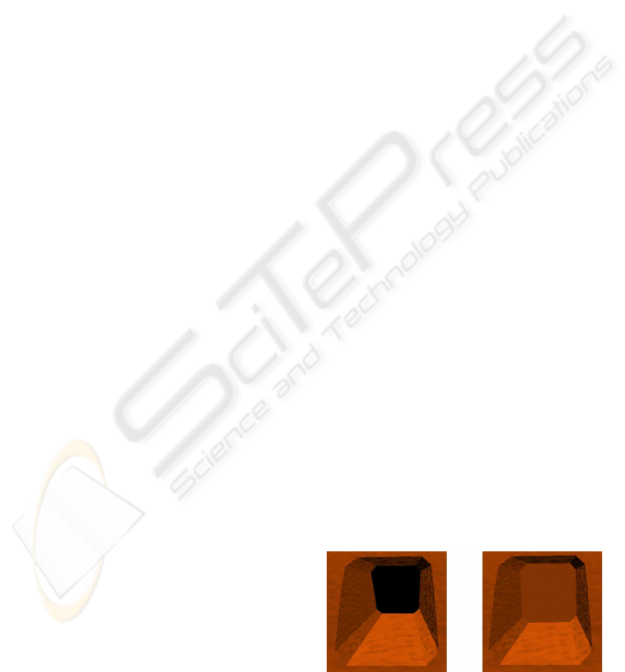
Carving events are deﬁned in two steps. First a

protovolume is deﬁned by sweeping a cross section

along a rectilinear axis. Then the carving is gener-

ated by subtracting the protovolume from the terrain

model.

The protovolume is characterized by two points,

a polygonal cross section, and two scalars. The two

points deﬁne both the axis and span of the protovol-

ume. The polygonal cross section deﬁnes the carv-

ing cross shape. Each scalar is used to scale respec-

tively the cross section to its actual size at the begin-

ning and at the end of the protovolume. The num-

ber of grounded heightmaps in a carving tunnel is the

number of sides in the polygonal cross section plus

two heightmaps that deﬁne the indoor-outdoor bor-

ders. The ground planes of these heightmaps are co-

incident with the XZ plane. In the carving cave, we

have one heightmap that deﬁnes the cave entry and

another one that deﬁnes the cave end. Carving events

can be applied only on the GHT root node since so

far we only support them on the XZ plane. Figure 9

left illustrates the shape generated by tunnel carving.

Figure 9 right depicts the shape generated by carving

a cave.

The carving process algorithm its outlined in Fig-

ure 10. First the algorithm extracts from the event

Figure 9: Carving events.

THE GROUNDED HEIGHTMAP TREE - A New Data Structure for Terrain Representation

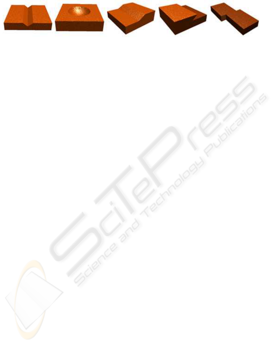
Figure 7: Geotectonic operations on GHT models.

procedure CarvingEvent(ght, e, newheightmaps)

BorderInnerNodes (newheightmaps, iheightmaps,

bheightmaps)

for hm in bheightmaps do

bound := ComputeBorderBoundary (ght, hm, e)

FillBorderData(ght, hm, e, bound)

LinkRootToBorder(ght, hm, e, bound)

UpdateHmap(ght, hm)

endfor

for hm in iheightmaps do

bound := ComputeInnerBoundary (ght, hm, e)

FillNoiseData(hm, bound)

endfor

LinkBorderToInner(bheightmaps, iheightmaps)

LinkRingInner(iheightmaps)

endprocedure

Figure 10: Carving process algorithm.

heightmaps,

newheightmaps

, those that deﬁne the

carving walls,

iheightmaps

, and the heightmaps of

the indoor-outdoor borders,

bheightmaps

For each indoor-outdoor border heightmap, ﬁrst

the set of cells that deﬁne the heights for the carving

cross section,

bound

, is computed. To preserve model

continuity, bound cells are linked to their neighbor

cells in

. Heightmap cells where the cross section is

projected are assigned as empty cells. After deﬁning a

border heightmap, those cells in

corresponding to

empty cells in the border heightmap must be labeled

as null links.

For each wall heightmap ﬁrst the set of cells that

deﬁnes the height values is computed. Then the

heights are deﬁned as a smooth noise.

Finally, to preserve continuity, border-inner and

inner-inner heightmaps links are established.

4 IMPLEMENTATION AND

RESULTS

The algorithms have been implemented on a Pen-

tium M 1.73 GHz, with 1GB RAM, nVidia Geforce

Go 6600 with 256 MB. The graphics API used was

OpenGL and the GLUT library was used for events

and window management. Digital elevation models

consisted of heightﬁelds with 128x128 cells.

To test the model performance, we haveconducted

two sets of experiments that we brieﬂy describe in

what follows. Related pictures and videos are avail-

able at (bib, ). The ﬁrst set of experiments consisted

in applying a number of single events, erosion and

faults, on a given terrain. Each event was applied on

a fresh terrain. Figure 11 illustrates the results gener-

ated by a linear erosion.

The second set of experiments included a number

of overlapping events applied in sequence to a given

terrain yielding a complex model. Figure 12 shows

on the top the set of ground planes on which the ter-

rain is built and, on the bottom the resulting terrain as

wireframe.

As a proof of concept, we have developed a small

application to edit a fresh terrain by applying radial

erosion. Each erosion is deﬁned as the result of crash-

ing a material particle on the terrain surface according

to a ﬁxed erosion law. A movie can be downloaded

from (bib, ).

5 CONCLUSIONS

In this work we have proposed the Grounded

Heightmaps Tree (GHT) as a new terrain model

which is a generalization of heightmaps that over-

comes limitations inherent to them like capturing ter-

rain overhangs and carvings.

Besides, we have deﬁned a set of operations to allow

editing the terrain. There are two families of opera-

tions: geotectonic events and carvings. The ﬁrst fam-

ily has been designed to mimic geotectonic eventslike

linear and radial erosion; normal, inverse and lateral

faults. The second family includes carving tunnels

and caves.

We have conducted a series of experiments to test the

model and associated operations performance. Pre-

liminary results show that they are both effective and

efﬁcient.

GRAPP 2008 - International Conference on Computer Graphics Theory and Applications

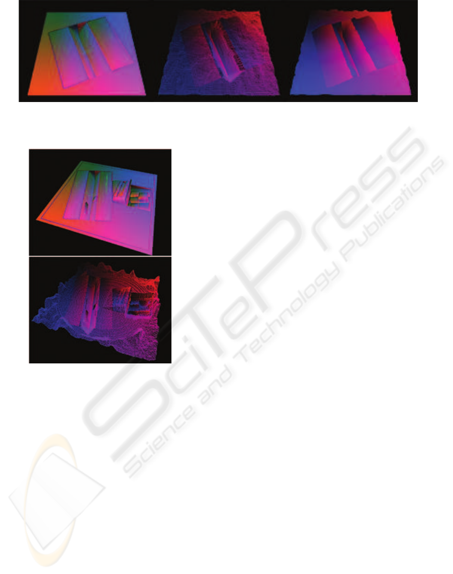
Figure 11: Linear erosion. Left) Ground heightmap planes. Middle) 3D wireframe view. Right) 3D solid view.

Figure 12: Complex model. Top) Set of ground planes

in the ﬁnal GHT. Bottom) Wire frame view after applying

some events.

ACKNOWLEDGEMENTS

This work has been partially funded by Ministerio

de Educaci´on y Ciencia and by FEDER under grant

TIN2004-06326-C03-01.

REFERENCES

The Grounded Heightmap Tree.

http://www.lsi.upc.edu/˜ jalonso/GHT.

Elias, H. http://freespace.virgin.net/hugo.elias.

Fault algorithm, T. http://www.lighthoused3d.com/opengl/terrain.

Klinkenberg, B. Digital elevation modeling.

http://www.geog.buffalo.edu/arcinfo/aiwwwtut/step3.html.

Martz, P. Generating random fractal terrain.

http://www.gameprogrammer.com/fractal.html.

Robot-frog. Terrain generation tutorial. http://www.robot-

frog.com/3d.

THE GROUNDED HEIGHTMAP TREE - A New Data Structure for Terrain Representation