
EFFICIENT INVERSE KINEMATICS ALGORITHM BASED ON
CONFORMAL GEOMETRIC ALGEBRA
Using Reconfigurable Hardware
Dietmar Hildenbrand
Research Center of Excellence for Computer Graphics, University of Technology, Darmstadt, Germany
Holger Lange, Florian Stock, Andreas Koch
Embedded Systems and Applications Group, University of Technology, Darmstadt, Germany
Keywords:
Geometric algebra, geometric computing, computer animation, inverse kinematics, hardware acceleration,
reconfigurable hardware, runtime performance.
Abstract:
This paper presents a very efficient approach for algorithms developed based on conformal geometric algebra
using reconfigurable hardware. We use the inverse kinematics of the arm of a virtual human as an example,
but we are convinced that this approach can be used in a wide field of computer animation applications. We
describe the original algorithm on a very high geometrically intuitive level as well as the resulting optimized
algorithm based on symbolic calculations of a computer algebra system. The main focus then is to demonstrate
our approach for the hardware implementation of this algorithm leading to a very efficient implementation.
1 INTRODUCTION
Based on an inverse kinematics application we show
that algorithms using the geometrically intuitive
mathematical language of conformal geometric alge-
bra can be implemented very efficiently using recon-
figurable hardware.
Our starting point is the inverse kinematics algo-
rithm for the arm of a virtual character of the paper
(Hildenbrand et al., 2006). It introduces the princi-
ple of optimizing geometric algebra algorithms using
the symbolic calculation feature of Maple. In sec-
tion 3 we present the optimized algorithm resulting
of this approach. In principle, we describe the algo-
rithm based on the computation of the coefficients of
the main data structure of conformal geometric alge-
bra, the 32-dimensional multivector. This kind of op-
timized algorithms uses only basic arithmetic opera-
tions.
These properties provide an adequate basis for our
hardware implementation as described in section 4.
The optimized algorithm of section 3 uses only oper-
ations easily performable by hardware and the com-
putations of the coefficients of the multivectors can be
executed in parallel. We use reconfigurable hardware
in order to have the chance to configure the hardware
acceleration depending on the application.
In a nutshell, the approach of this paper promises
to combine the easy development of algorithms based
on conformal geometric algebra with very efficient
implementations in a wide field of computer anima-
tion and computer graphics applications.
2 CONFORMAL GEOMETRIC
ALGEBRA
Blades are the basic computational elements and the
basic geometric entities of the geometric algebra. For
example, the 5D Conformal Geometric Algebra pro-
vides a great variety of basic geometric entities to
compute with. It consists of blades with grades 0, 1,
2, 3, 4 and 5, whereby a scalar is a 0-blade (blade of
grade 0). There exists only one element of grade five
in the Conformal Geometric Algebra. It is therefore
also called the pseudoscalar. A linear combination of
blades is called a k-vector. So a bivector is a linear
combination of blades with grade 2. Other k-vectors
are vectors (grade 1), trivectors (grade 3) and quad-
vectors (grade 4). Furthermore, a linear combination
of blades of different grades is called a multivector.
Multivectors are the general elements of a Geometric
Algebra. Table 2 lists all the 32 blades of Conformal
300
Hildenbrand D., Lange H., Stock F. and Koch A. (2008).
EFFICIENT INVERSE KINEMATICS ALGORITHM BASED ON CONFORMAL GEOMETRIC ALGEBRA - Using Reconfigurable Hardware.
In Proceedings of the Third International Conference on Computer Graphics Theory and Applications, pages 300-307
DOI: 10.5220/0001094603000307
Copyright
c
SciTePress
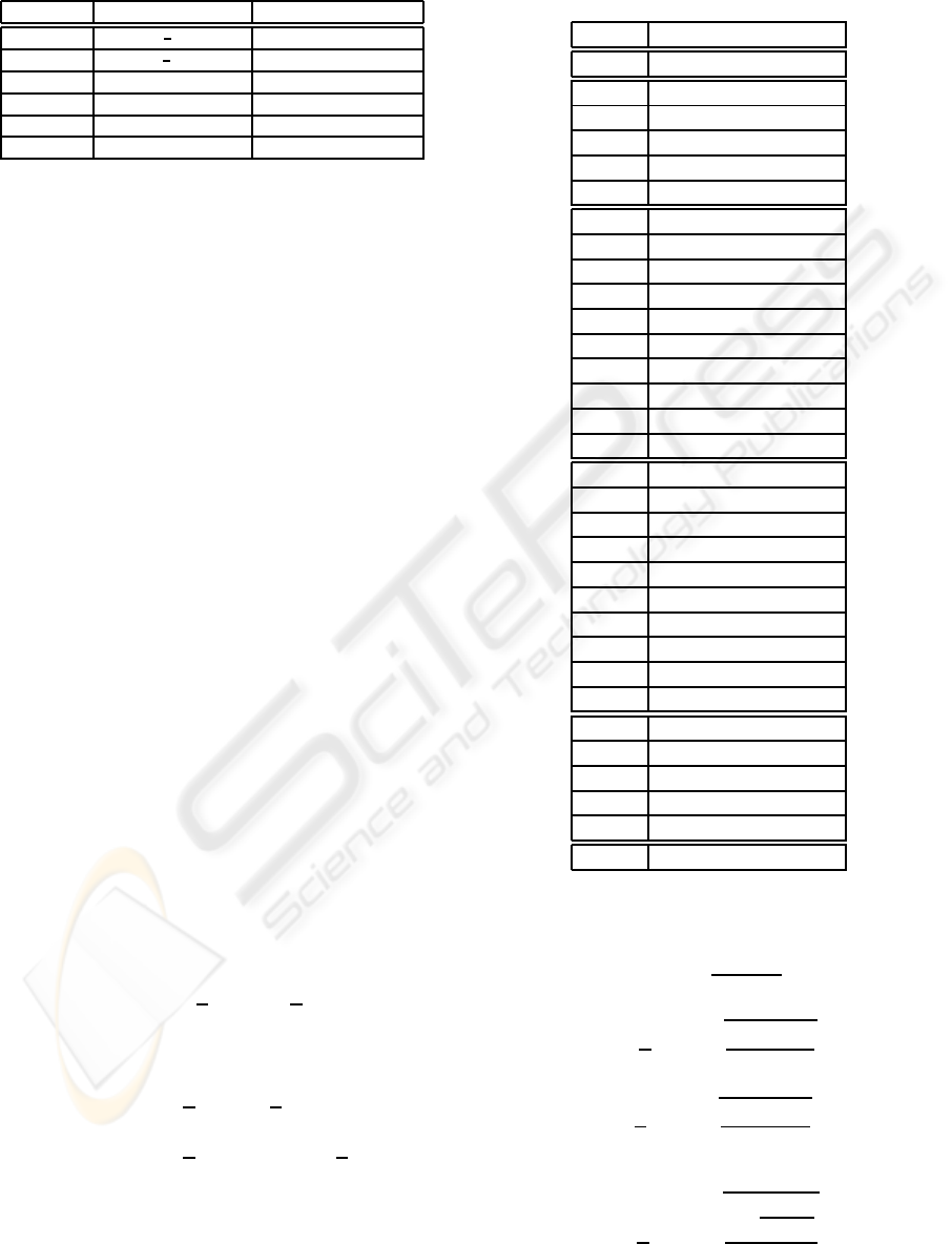
Table 1: Representations of the conformal geometric enti-
ties.
entity standard repr. direct repr.
Point P = x+
1
2
x
2
e
∞
+ e
0
Sphere s = P−
1
2
r
2
e
∞
s
∗
= x
1
∧x
2
∧x
3
∧x
4
Plane π = n+ de
∞
π
∗
= x
1
∧x
2
∧x
3
∧e
∞
Circle z = s
1
∧s
2
z
∗
= x
1
∧x
2
∧x
3
Line l = π
1
∧π
1
l
∗
= x
1
∧x
2
∧e
∞
Point Pair P
p
= s
1
∧s
2
∧s
3
P
∗
p
= x
1
∧x
2
Geometric Algebra. The indices indicate 1: scalar,
2..6: vector 7..16: bivector, 17..26: trivector, 27..31:
quadvector, 32: pseudoscalar.
Table 1 presents the basic geometric entities of
conformal geometric algebra, points, spheres, planes,
circles, lines and point pairs. The s
i
represent differ-
ent spheres and the π
i
different planes. The two rep-
resentations are dual to each other. In order to switch
between the two representations, the dual operator
which is indicated by ’
∗
’, can be used. For example
in the standard representation a sphere is represented
with the help of its center point P and its radius r,
while in the direct representation it is constructed by
the outer product ’∧’ of four points x
i
that lie on the
surface of the sphere (x
1
∧x
2
∧x
3
∧x
4
). In standard
representation the dual meaning of the outer product
is the intersection of geometric entities. For example
a circle is defined by the intersection of two spheres
(s
1
∧s
2
).
Quaternions are embedded in the Conformal Ge-
ometric Algebra in a very intuitive way. The main
observation is that an arbitrary line through the origin
represents the rotation axis for a quaternion if we use
the following definitions for the imaginary units
i = e
3
∧e
2
, (1)
j = e
1
∧e
3
, (2)
k = e
2
∧e
1
. (3)
A rotation around the line L as nomalized rotation
axis with an angle of φ can be computed as the fol-
lowing quaternion:
Q = cos(
φ
2
) + Lsin(
φ
2
) (4)
For example, if L = i = e
3
∧e
2
, the resulting quater-
nion
Q = cos(
φ
2
) + isin(
φ
2
)
= cos(
φ
2
) + (e
3
∧e
2
)sin(
φ
2
)
represents a rotation around the x-axis. For efficiency
reasons we use an approach to calculate quaternions
without the need of using trigonometric functions.
Table 2: A multivector in the 5D Conformal Geometric Al-
gebra is a linear combination of 32 blades. On hardware all
its coefficients can be computed in parallel.
Index blade
1 1
2 e
1
3 e
2
4 e
3
5 e
∞
6 e
0
7 e
1
∧e
2
8 e
1
∧e
3
9 e
1
∧e
∞
10 e
1
∧e
0
11 e
2
∧e
3
12 e
2
∧e
∞
13 e
2
∧e
0
14 e
3
∧e
∞
15 e
3
∧e
0
16 e
∞
∧e
0
17 e
1
∧e
2
∧e
3
18 e
1
∧e
2
∧e
∞
19 e
1
∧e
2
∧e
0
20 e
1
∧e
3
∧e
∞
21 e
1
∧e
3
∧e
0
22 e
1
∧e
∞
∧e
0
23 e
2
∧e
3
∧e
∞
24 e
2
∧e
3
∧e
0
25 e
2
∧e
∞
∧e
0
26 e
3
∧e
∞
∧e
0
27 e
1
∧e
2
∧e
3
∧e
∞
28 e
1
∧e
2
∧e
3
∧e
0
29 e
1
∧e
2
∧e
∞
∧e
0
30 e
1
∧e
3
∧e
∞
∧e
0
31 e
2
∧e
3
∧e
∞
∧e
0
32 e
1
∧e
2
∧e
3
∧e
∞
∧e
0
The angle between two lines or two planes is defined
as follows:
cos(θ) =
o
∗
1
·o
∗
2
o
∗
1
o
∗
2
, (5)
cos(
φ
2
) = ±
r
1+ cos(φ)
2
(6)
and
sin(
φ
2
) = ±
r
1−cos(φ)
2
, (7)
leading to the formulas
cos(
φ
2
) = ±
v
u
u
t
1+
o
∗
1
·o
∗
2
|
o
∗
1
||
o
∗
2
|
2
(8)
EFFICIENT INVERSE KINEMATICS ALGORITHM BASED ON CONFORMAL GEOMETRIC ALGEBRA - Using
Reconfigurable Hardware
301
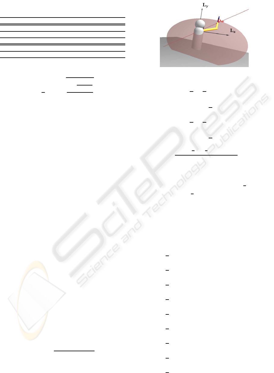
Table 3: Input/output parameters of the inverse kinematics
algorithm.
parameter meaning
P
w
target point of wrist
φ swivel angle
d
1
,d
2
length of the forearm and the upper arm
Q
s
shoulder quaternion
Q
e
elbow quaternion
and
sin(
φ
2
) = ±
v
u
u
t
1−
o
∗
1
·o
∗
2
|
o
∗
1
||
o
∗
2
|
2
(9)
The signs of these formulas depend on the applica-
tion.
For the foundations of conformal geometric al-
gebra and its application to kinematics please refer
for instance to (L.Dorst et al., 2007), (Rosenhahn,
2003), (Bayro-Corrochano and Zamora-Esquivel,
2004), (Hildenbrand et al., 2005) and to the tutorials
(Hildenbrand et al., 2004) and (Hildenbrand, 2005).
3 THE OPTIMIZED INVERSE
KINEMATICS ALGORITHM
In this section we present the optimized inverse kine-
matics algorithm for the arm of a virtual character as
described in (Hildenbrand et al., 2006). We especially
use its optimization approach based on Maple in or-
der to get the most elementary relationship between
the input and output parameters of the algorithm.
The goal of the inverse kinematics algorithm is to
compute the quaternions Q
s
and Q
e
based on the tar-
get point P
w
and the parameters φ,d
1
,d
2
(see table 3).
3.1 Compute the Swivel Plane
First of all, we compute the swivel plane. Accord-
ing to (Tolani et al., 2000) we use the swivel angle φ
as one free degree of redundancy. The swivel plane
is the plane rotated by φ around the line L
sw
through
shoulder (at the origin) and P
w
(see figure 1).
The length of L
sw
can be computed as
|L
sw
| =
q
p
w
2
x
+ p
w
2
y
+ p
w
2
z
. (10)
The coefficients of the swivel plane optimized by
Maple are:
Figure 1: Swivel plane.
π
swivel
x
=(2cos
φ
2
sin
φ
2
p
w
z
p
w
x
− p
w
y
|L
sw
|+
2p
w
y
|L
sw
|cos
φ
2
2
)/|L
sw
|
π
swivel
y
=(2cos
φ
2
sin
φ
2
p
w
z
p
w
y
+ p
w
x
|L
sw
|−
2p
w
x
|L
sw
|cos
φ
2
2
)/|L
sw
|
π
swivel
z
=
−2sin
φ
2
cos
φ
2
(p
w
2
x
+ p
w
2
y
)
|L
sw
|
(11)
3.2 The Elbow Point P
e
With the help of the two spheres S
1
= P
w
−
1
2
d
2
2
e
∞
and
the sphere S
2
= e
o
−
1
2
d
2
1
e
∞
with center points P
w
and
e
o
and radii d
2
,d
1
we are able to compute the circle
Z
e
= S
1
∧S
2
determining all the possible locations of
the elbow as the intersection of the spheres (see table
1).The intersection with the swivel plane delivers the
point pair Pp = Z
e
∧π
swivel
.
Its coefficients based on the optimizations of
Maple are as follows
PP
i
=
1
2
π
swivel
x
(p
w
2
x
+ p
w
2
z
+ p
w
2
y
+ d
2
1
−d
2
2
)
PP
j
=
1
2
π
swivel
y
(p
w
2
x
+ p
w
2
z
+ p
w
2
y
+ d
2
1
−d
2
2
)
PP
k
=
1
2
π
swivel
z
(p
w
2
x
+ p
w
2
z
+ p
w
2
y
+ d
2
1
−d
2
2
)
PP
14
=
1
2
(1−d
2
1
)(p
w
y
π
swivel
z
− p
w
z
π
swivel
y
)
PP
15
=
1
2
(1+ d
2
1
)(p
w
z
π
swivel
y
− p
w
y
π
swivel
z
)
PP
24
=
1
2
(1−d
2
1
)(p
w
z
π
swivel
x
− p
w
x
π
swivel
z
)
PP
25
=
1
2
(1+ d
2
1
)(p
w
x
π
swivel
z
− p
w
z
π
swivel
x
)
PP
34
=
1
2
(d
2
1
−1)(p
w
y
π
swivel
x
− p
w
x
π
swivel
y
)
PP
35
=
1
2
(1+ d
2
1
)(p
w
y
π
swivel
x
− p
w
x
π
swivel
y
) (12)
GRAPP 2008 - International Conference on Computer Graphics Theory and Applications
302
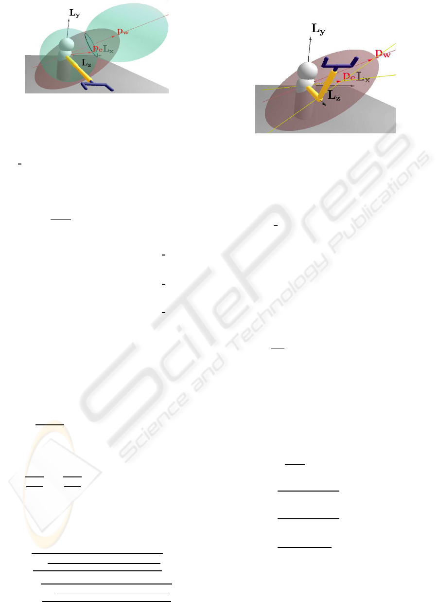
Figure 2: Compute the elbow point.
We decide for one of the two possible elbow
points and compute the three components of the el-
bow point p
e
x
, p
e
y
, p
e
z
from the point pair PP:
einf PP =(PP
35
−PP
34
)
2
+ (PP
14
−PP
15
)
2
+ (PP
25
−PP
24
)
2
tmp
1
= −PP
2
i
−PP
2
j
−PP
2
k
−PP
2
14
+
PP
2
15
−PP
2
24
+ PP
2
25
−PP
2
34
+ PP
2
35
tmp
sqrt
=
√
tmp
1
p
e
x
=(PP
j
(PP
34
−PP
35
) + PP
k
(PP
25
−PP
24
+ tmp
sqrt
(PP
15
−PP
14
))/einf PP
p
e
y
=(PP
i
(PP
35
−PP
34
) + PP
k
(PP
14
−PP
15
)
+ tmp
sqrt
(PP
25
−PP
24
))/einf PP
p
e
z
=(PP
j
(PP
15
−PP
14
) + PP
i
(PP
24
−PP
25
)
+ tmp
sqrt
(PP
35
−PP
34
))/einf PP (13)
3.3 Calculate the Elbow Quaternion Q
e
The elbow angle θ
4
is computed with the help of the
line L
se
= (e
o
∧P
e
∧e
∞
)
∗
through the shoulder and
the elbow and the line L
ew
= (P
e
∧P
w
∧e
∞
)
∗
through
the shoulder and the wrist. Based on these two lines
we are able to compute the angle between them (c
4
=
cos(θ
4
) =
L
∗
se
·L
∗
ew
|L
∗
se
||L
∗
ew
|
) according to equation (5).
Now, we are able to compute the quaternion Q
e
=
cos(θ
4
/2) + sin(θ
4
/2)i according to equation (1). It
represents a rotation around the local x-axis with the
angle θ
4
. The optimized version of this quaternion is
Q
e
=
q
1+c
4
2
−
q
1−c
4
2
i, according to (8) and (9).
This quaternion rotates the upper arm correspond-
ing to the angle between the two yellow lines as
shown in fig. 3.
The quaternion Q
e
of the rotation at the elbow
joint:
Q
e
=
s
1+
p
e
2
x
−p
e
x
p
w
x
+p
e
2
y
−p
e
y
p
w
y
−p
e
z
p
w
z
+p
e
2
z
d
1
d
2
2
−
s
1−
p
e
2
x
−p
e
x
p
w
x
+p
e
2
y
−p
e
y
p
w
y
−p
e
z
p
w
z
+p
e
2
z
d
1
d
2
2
i (14)
Figure 3: Use the elbow quaternion.
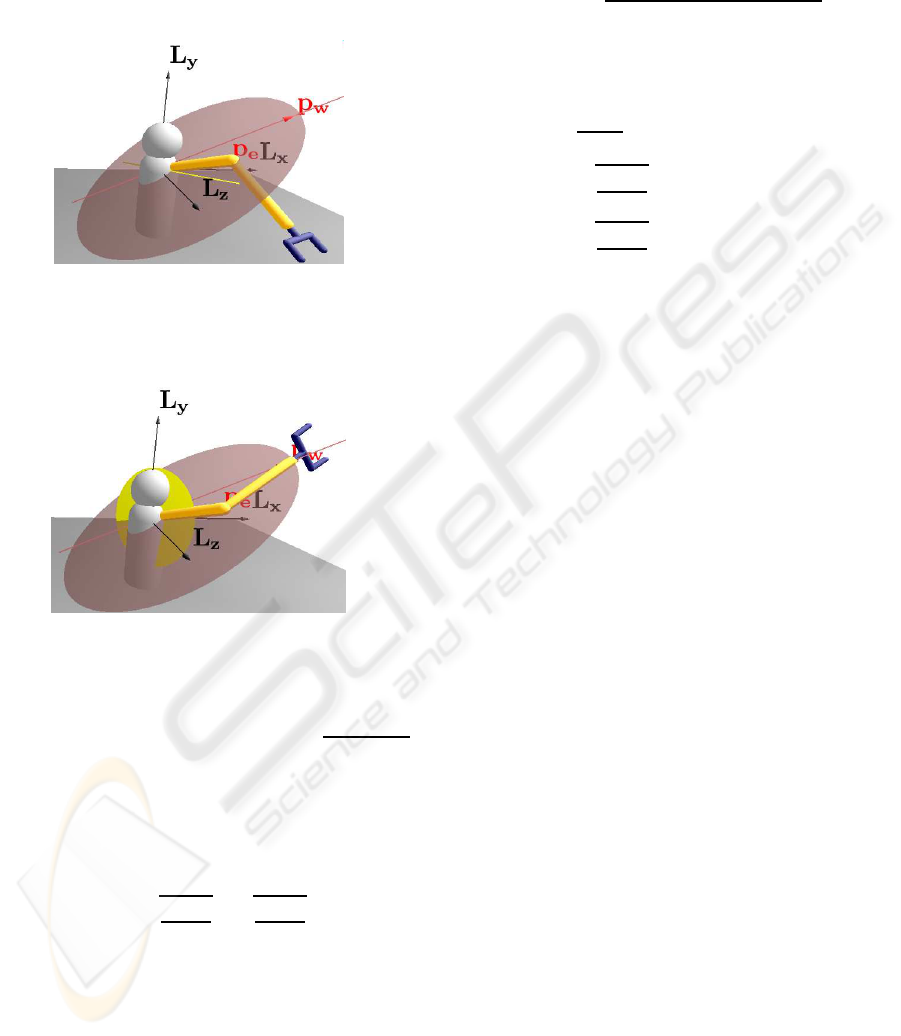
3.4 Rotate to the Elbow Position
At first we calculate the middle line L
m
through the
origin within the same distance from the points P
e
and
P
ze
= d
1
e
3
+
1
2
d
2
1
e
∞
+ e
o
. We will need this line L
m
in
the next step in order to rotate around this line.
To compute L
m
, we use the middle plane as the
difference of the two points P
e
and P
ze
(π
m
= P
ze
−P
e
)
and the plane through the origin and the points P
e
and P
ze
as π
∗
e
= e
o
∧P
ze
∧P
e
∧e
∞
and intersect them
(L
m
= π
e
∧π
m
).
In order to rotate the elbow towards our already
computed point P
e
we have to rotate around the mid-
dle line of the previous step with angle π. This results
in a quaternion identical with the normalized middle
line (Q
12
=
L
m
|L
m
|
). Figure 4 shows this rotation from
the z-axis L
z
to the elbow point with the help of the
yellow middle line.
The result for the quaternion Q
12
optimized by
Maple can be computed as follows:
tmp
2
=d
4
1
p
e
2
y
−2d
3
1
p
e
2
y
p
e
z
+ d
2
1
p
e
2
y
p
e
2
z
+
d
4
1
p
e
2
x
−2d
3
1
p
e
2
x
p
e
z
+ d
2
1
p
e
2
x
p
e
2
z
+
d
2
1
p
e
4
x
+ 2d
2
1
p
e
2
x
p
e
2
y
+ d
2
1
p
e
4
y
|L
m
| =
√
tmp
2
q
12
i
=
d
1
p
e
x
(d
1
− p
e
z
)
|L
m
|
q
12
j
=
d
1
p
e
y
(d
1
− p
e
z
)
|L
m
|
q
12
k
=
d
1
(p
e
2
x
+ p
e
2
y
)
|L
m
|
(15)
3.5 Rotate to the Wrist Location
The angle θ
3
(and the resulting quaternion Q
3
) is
computed with the help of the y-z-plane rotated by
EFFICIENT INVERSE KINEMATICS ALGORITHM BASED ON CONFORMAL GEOMETRIC ALGEBRA - Using
Reconfigurable Hardware
303
the quaternion Q
12
and the swivel plane. The plane
in y and z direction (with normal vector e
1
and zero
distance to the origin), is computed by π
yz
= e
1
. The
rotated plane π
yz2
results in π
yz2
= Q
12
π
yz
˜
Q
12
.
Figure 4: Rotate to the elbow position.
Figure 5: Rotate to the wrist location.
Based on these two planes we are able to compute
the angle between them as c
3
= cos(θ
3
) =
π
∗
yz2
·π
∗
swivel
π
∗
yz2
|
π
∗
swivel
|
according to equation (5) and we get the quaternion
Q
3
= cos(θ
3
/2) + sin(θ
3
/2)k. It represents a rotation
around the local z-axis with the angle θ
3
. The opti-
mized version of this quaternion is
Q
3
= ±
r
1+ c
3
2
+
r
1−c
3
2
k, (16)
according to (8) and (9).
Note: the sign of this quaternion depends on which
side of the plane π
yz2
the point P
w
is lying. This can
be easily computed with the help of the inner product
π
yz2
·P
w
. This quaternion rotates the arm to the wrist
location as shown in figure 5.
The rotation at the shoulder joint optimized by
Maple can be computed as follows:
c
3
=(π
swivel
x
(q
12
2
k
+ q
12
2
j
−q
12
2
i
)−
2q
12
i
(q
12
j
π
swivel
y
+ q
12
k
π
swivel
z
))
/
q
π
swivel
2
x
+ π
swivel
2
y
+ π
swivel
2
z
sign =p
w
x
(q
12
2
i
−q
12
2
k
−q
12
2
j
)+
2q
12
i
(q
12
k
p
w
z
+ q
12
j
p
w
y
)
sign =
sign
|sign|
q
3
scalar
=
r
1+ c
3
2
q
3
k
=
r
1−c
3
2
sign (17)
The resulting quaternion for the shoulder rotation
can now be computed as the product Q
s
= Q
12
Q
3
. The
final result of Q
s
optimized by Maple can be com-
puted as follows:
Q
s
= −q
12
k
·q
3
k
+
(q
12
i
·q
3
scalar
+ q
12
j
·q
3
k
)i−
(q
12
i
·q
3
k
−q
12
j
·q
3
scalar
) j+
(q
12
k
·q
3
scalar
)k (18)
4 HARDWARE
IMPLEMENTATION
The previous section describes the inverse kinemat-
ics algorithm, originally developed based on confor-
mal geometric algebra, with the help of the equations
(10) to (18) using only basic arithmetic operations. In
principle they describe the computation of the compo-
nents of the 32-dimensional multivectors of the alge-
bra. Equation (12) for instance computes the 9 com-
ponents of a point pair. On hardware all these compu-
tations can be executed in parallel.
These equations provide an adequate basis for the
following hardware implementation.
4.1 The Hardware Platform
The accelerated hardware implementation targets a
Field Programmable Gate Array (FPGA). These re-
configurabledevicesallow the implementationof cus-
tom circuits, but provide only limited resources. The
Xilinx Virtex 2/4 series of FPGAs comprises an ar-
ray of lookup-tables (LUTs) with one associated Flip-
Flop (FF) per LUT. Each LUT can implement an arbi-
trary function of up to four independent 1-bit inputs.
GRAPP 2008 - International Conference on Computer Graphics Theory and Applications
304

Table 4: Comparison of required operations.
+, − ×
√
a
b
,
1
b
unoptimzed 147 87 8 16
optimized 69 42 8 10
To fit the calculation on the FPGA and speed it
up, we decided to use only fixed point calculations in-
stead of floating point operations (which is possible
but not as efficient as fixed point). As a side effect of
calculating in dedicated hardware, the cost of opera-
tions drastically changes: e.g. multiplication and ad-
dition need the same calculation time, whereas recip-
rocal value, division and square root are really costly
in both execution time and FPGA resources.
4.2 Preparatory Optimization
The equations described in the previous section were
the starting point for further optimization. They
where manually optimized to reduce the number of
operations, especially the expensive ones. E.g. we
changed the last six equations of (12) to
PP
+
m
= PP
m5
+ PP
m4
= 2d
2
1
(p
w
...
π
swivel
...
− p
w
...
π
swivel
...
)
PP
−
m
= PP
m5
−PP
m4
= 2(p
w
...
π
swivel
...
− p
w
...
π
swivel
...
) (19)
m = 1,2,3
These six equations comprise the same number of
(constant) multiplications and additions, so the calcu-
lations seem as expensive as before. However, now
the PP
+
m
and PP
−
m
share a common subexpression,
so 2 multiplications and 1 addition are saved. Fur-
thermore, the constant multiplication in PP
+
m
is now
a constant multiplication with a power of 2, which
is implemented in hardware efficiently through sim-
ply shifting wire connections by the exponent value.
Since only pure wiring is involved, no additional
ressources are required for this kind of multiplication.
In the following computation of the elbow points
in (13), the frequent reference to PP
m4
and PP
m5
is
clearly obvious. However, as the references occur
only in a sum or difference, the new PP
+
m
and PP
−
m
can be used instead, thus eliminating an addition each
time. Only tmp
1
does not refer directly to a sum or
difference, but it can be expressed as
tmp
1
= ... + PP
+
m
PP
−
m
+ .. .,
eliminating another 3 multiplications and 3 additions.
For a comparison of the required operations be-
fore and after optimization see table 4.
4.3 Fixed Point Conversion
The optimized equations from the previous sec-
tion (4.2) were manually transformed into dataflow
graphs. For conversion into fixed point format suit-
able for efficient hardware realization, we need to de-
fine an as small as possible word length for every
variable and intermediate result in these graphs (e.g.,
see figure 6 calculation of p
e
x
from equation (13) ).
While automatic conversions from floating point to
fixed point exist (Han, 2006), we preferred a manual
translation nevertheless, as automatic conversions are
still limited (e.g. not all operationsare supported). We
used two approaches for minimizing the word length
while retaining sufficient precision.
Analytic approach: The input parameters have
a given precision and value range which were propa-
gated forward through the data flow graphs. On the
other hand, the expected precision and value range of
the result were propagated backwards (e.g. the pre-
cision of a sum is the maximum of the precision of
the summands). Figure 6 shows the resulting value
ranges as annotations to the nodes.
Moreover, we can benefit from dedicated knowl-
edge of the problem and inequalities to narrow the
value range even further. Referring to the graph in
figure 6, we know that the resulting point p
e
x
is the
elbow. Hence, the distance is given by d
1
, which also
implies that |p
e
x
| ≤ d
1
, |p
e
y
| ≤ d
1
and |p
e
z
| ≤ d
1
(nar-
rowed value ranges are shown inside dashed frames at
the nodes in figure 6).
Empiric approach: To verify the analytical anal-
ysis (and obtain results where the analytic approach
fails), all graphs were implementedin MATLAB. Then
random valid values were supplied as inputs to the
equations, which were calculated subsequently with
default Matlab double precision (= 64 bits) floating
point arithmetic as well as the Fixed-Point Toolbox
(The MathWorks, 2007). The Fixed-Point Toolbox
allows exact specification of the number format used
for fixed point arithmetic (sign bit, integer and frac-
tional word length) for each variable.
The analyses show that it is sufficient to use a total
word length of 32 bits or less.
4.4 Hardware Realization
The dataflow graphs were implemented as a fully
spatial pipeline in the hardware description language
Verilog. Spatial parallelism means parallel execu-
tion of operations that can be performed simultane-
ously due to independent subexpressions. Pipelin-
ing further extends parallel execution to simultane-
ous calculation of sequentially dependent operations.
EFFICIENT INVERSE KINEMATICS ALGORITHM BASED ON CONFORMAL GEOMETRIC ALGEBRA - Using
Reconfigurable Hardware
305
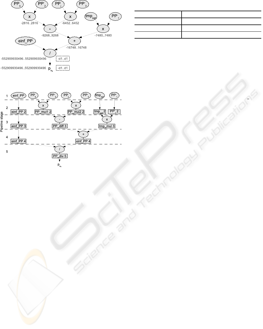
Figure 6: Dataflow graph for p
ex
.
Figure 7: Pipeline schedule for p
ex
(cf. figure 6).
To this end, the parallel-sequential dataflow graph is
partitioned into many sequential execution steps, also
known as pipeline stages. The results of the first ex-
ecution step are used as inputs for the second step.
This scheme is repeated for all subsequent operation
steps. Hence, parallel execution for all operations is
exploited if possible.
As a benefit, the execution time for each pipeline
stage is minimized with respect to the whole sequen-
tial dataflow graph. The faster pipeline stages, execut-
ing in parallel, allow for a higher clock frequency of
the hardware, thus increasing overall throughput with
a set of results delivered at each clock cycle. The la-
tency is only experienced twice at pipeline startup and
shutdown, or respectively, in single shot mode.
We chose to optimize the pipeline for maximum
throughput to demonstrate the potential of acceler-
ating the algorithm in hardware. Nevertheless other
optimization goals (minimum use of hardware re-
sources/area, low latency, low power consumption)
are possible as well, but not discussed here.
Many subexpression trees have different heights
which mostly correspond to inhomogeneous numbers
of pipeline stages from common input values to in-
termediate values, the latter to be merged for subse-
quent calculations. To account for this difference, the
Table 5: Hardware mapping results.
Number of LUTs ≈ 30000 (45% of 2VP70 max.)
Clock frequency 100 MHz
Throughput 1 set of results per clock cycle
Latency ≈ 550 clock cycles
pipeline was balanced with additional flip-flop stages
on the shorter subtrees, hence providing intermediate
results synchronouslyat such merge points. The exact
pipline timing (also known as schedule) for p
ex
(cf.
13) is shown in figure 7. The rectangles represent flip-
flops which temporarily store the intermediate results
of the 5 pipline stages (separated by dashed horizon-
tal lines). Note the balancing flip-flops for ein f PP,
tmp
sqrt
and PP
−
1
.
In contrast to a fully spatial pipeline which is cus-
tomized for the specific application, general purpose
instruction-based execution models as employed in
CPUs or Digital Signal Processors (DSPs) only pro-
vide for a very limited exploitation of both spatial
and sequential (pipelining) parallelism. E.g., a CPU
pipeline has to be flushed and refilled on every (un-
predicted) branch in the control flow of the software
code. What is more, even a superscalar CPU hardly
executes more than half a dozen instructions per clock
cycle (Hennessy and Patterson, 2007, chapter 3.6).
5 RESULTS
The Verilog HDL description of the dataflow graph
was mapped to a Xilinx Virtex 2VP70 FPGA (Xil-
inx, 2005) using the Xilinx ISE tools. For synthesis,
we generated dedicated dividers and squareroot cores
with the Xilinx Core Generator (part of the ISE tools).
Multiplications were automatically mapped to multi-
plier units, which are specialized, non-reconfigurable
fast hardware blocks provided within the FPGA fab-
ric. Table 5 shows the mapping and performance re-
sults for the complete dataflow graph.
Our test scenario was the computation of the mo-
tion of the arm of the virtual character based on 100
steps of inverse kinematics computations. To evalu-
ate the hardware performance compared with a pure
software implementation, 100 data sets residing in
main memory which represent target points in space
are converted to quaternions by both our fully spa-
tial pipeline running at 100 MHz clock speed and a
Intel Centrino M715CPU running at 1.5 GHz. After
conversion, the resulting data sets are written back to
memory. Table 6 shows the accelerated HW and pure
SW execution times.
GRAPP 2008 - International Conference on Computer Graphics Theory and Applications
306

Table 6: SW and HW execution times for 100 data sets.
execution time
SW on CPU 860 us
HW pipeline 6 us
(5 us until first data set +
100 * 10 ns remaining sets)
6 COMPARISON TO GPU
REALISATION
The fined-grained parallelism exploited by our FPGA
realisation is very different from the coarser-grained
one accessible when implementing the algorithm on a
modern GPU. A typical example, such as the NVidia
G80 architecture (NVIDIA Corp., 2007), can process
just 128 operations in parallel, using a SIMD (small-
vector) paradigm. In our approach, however, each of
the 550 pipeline stages has 4.. .10 operatorsexecuting
in parallel, leading to a total parallelism of thousands
of operations. Additionally, the GPU processing ele-
ments have a fixed architecture and cannot be tailored
to specific constants or precision requirements. Fur-
thermore, the GPU computation has to be manually
partitioned into units of parallel execution (so-called
threads or warps). In our approach, the mathemat-
ical formulation itself directly determines the hard-
ware structure of the accelerator, no additional par-
titioning is required. While we have not implemented
the algorithm on such a GPU yet, we expect the FPGA
realisation (especially one using a more recent chip
than the one in the current prototype) to be competi-
tive with a modern GPU implementation despite the
clock speed differences (550 MHz FPGA vs. 1350
MHz GPU). Such an evaluation is planned in a fur-
ther refinement of this work.
7 CONCLUSIONS
We presented a way to implement algorithms based
on conformal geometric algebra on hardware. After
having developed an algorithm easy and geometri-
cally intuitive on a very high level we are using the
symbolic calculation functionality of Maple as a soft-
ware optimization procedure. While this approach is
already leading to very efficient code we presented an
approach to further improve the performance using
configurable hardware. This implementation turned
out to be more than 100 times faster. These results
were shown based on an inverse kinematics algorithm
but we are convinced that this approach can be used
very advantageously in a lot of computer animation
and computer graphics applications.
REFERENCES
Bayro-Corrochano, E. and Zamora-Esquivel, J. (2004). In-
verse kinematics, fixation and grasping using confor-
mal geometric algebra. In IROS 2004, September
2004, Sendai, Japan.
Han, K. (2006). Automating Transformations from
Floating-point to Fixed-point for Implementing Dig-
ital Signal Processing Algorithms. PhD thesis, Dept.
of Electrical and Computer Engineering, The Univer-
sity of Texas at Austin.
Hennessy, J. L. and Patterson, D. A. (2007). Computer ar-
chitecture. Kaufmann [u.a.], Amsterdam [u.a.].
Hildenbrand, D. (2005). Geometric computing in computer
graphics using conformal geometric algebra. Comput-
ers & Graphics, 29(5):802–810.
Hildenbrand, D., Bayro-Corrochano, E., and Zamora-
Esquivel, J. (2005). Advanced geometric approach for
graphics and visual guided robot object manipulation.
In proceedings of ICRA conference, Barcelona, Spain.
Hildenbrand, D., Fontijne, D., Perwass, C., and Dorst, L.
(2004). Tutorial geometric algebra and its applica-
tion to computer graphics. In Eurographics confer-
ence Grenoble.
Hildenbrand, D., Fontijne, D., Wang, Y., Alexa, M., and
Dorst, L. (2006). Competitive runtime performance
for inverse kinematics algorithms using conformal ge-
ometric algebra. In Eurographics conference Vienna.
L.Dorst, Fontijne, D., Mann, S., and Kaufman, M. (2007).
Geometric Algebra for Computer Science, An Object-
Oriented Approach to Geometry. Morgan Kaufman.
NVIDIA Corp. (2007). NVIDIA CUDA Compute Unified
Device Architecture Programming Guide Version 1.0.
NVIDIA Corp.
Rosenhahn, B. (2003). Pose Estimation Revisited. PhD
thesis, Inst. f. Informatik u. Prakt. Mathematik der
Christian-Albrechts-Universit¨at zu Kiel.
The MathWorks (2007). Fixed-Point Toolbox 2, Reference.
The MathWorks.
Tolani, D., Goswami, A., and Badler, N. I. (2000). Real-
time inverse kinematics techniques for anthropomor-
phic limbs. Graphical Models, 62(5):353–388.
Xilinx (2005). Virtex-II Pro and Virtex-II Pro X Platform
FPGAs: Complete Data Sheet (DS083). Xilinx.
EFFICIENT INVERSE KINEMATICS ALGORITHM BASED ON CONFORMAL GEOMETRIC ALGEBRA - Using
Reconfigurable Hardware
307
