
SURF
ACE-SURFACE INTERSECTION BY
HERMITE INTERPOLATION
Eng-Wee Chionh
School of Computing, National University of Singapore, Republic of Singapore 117590
Keywords:
Hermite interpolation, surface-surface intersection.
Abstract:
A fast heuristic to approximate the intersection curve of two surface patches was originally proposed by
Sederberg and Nishita. The patches are rationally parametrized and they cut each other transversely. This
paper reports a simple generalization that greatly improves the accuracy of the original heuristic. The general-
ization either avoids or attenuates the approximation error. Avoidance is achieved when the improved heuristic
produces the exact intersection curve; attenuation is accomplished with an aggregate square distance formula
guiding the selection of a generalized constraint for a better fit.
1 INTRODUCTION
Finding the intersection curve of two surfaces is a fun-
damental operation in computer graphics and com-
puter geometric design and processing (Song et al.,
2004). It is an intrinsically difficult problem and ex-
pectedly solutions depend on the surface description.
In the realm of rationally parametrized surfaces, this
difficulty is apparent because the intersection curve
degree can be very high even when the surface de-
grees are modest. Recall that the degree of a curve in
3-space is the number of times it intersects a general
plane. By Bezout’s theorem (Cox et al., 1998), the
degree of the intersection curve of two general tensor
product surfaces of bi-degrees m
1
× m
2
and n
1
× n
2
is 4m
1
m
2
n
1
n
2
, and that of two general triangular sur-
faces of total degrees m and n is m
2
n
2
. For the popu-
lar bi-cubic surface patches in computer geometry, the
intersection curve degree works out to be 324! What
is worst, the intersection curve of two rational sur-
faces need not be rational. It is well known that an
algebraic curve is rational if and only if its genus is
zero (Fulton, 1969). Katz and Sederberg (Katz and
Sederberg, 1988) show that the genus g of the inter-
section curve of two general tensor product surfaces
of parametric bi-degrees m
1
× m
2
and n
1
× n
2
is
g = 8m
1
m
2
n
1
n
2
− 2m
1
m
2
(n
1
+ n
2
)
−2n
1
n
2
(m
1
+ m
2
) + 1; (1)
and that of two general triangular surfaces of paramet-
ric total degrees m and n is
g = 2m
2
n
2
−
3
2
m
2
n −
3
2
n
2
m +1. (2)
Thus
in general the intersection curve of two bi-
degree surfaces is non-rational and that of two trian-
gular surfaces is rational if and only if one is a plane
and the other is either a plane or a quadric surface.
Currently, the many existing methods for finding
the intersection curve of two surfaces may be broadly
classified under either geometric subdivision or topo-
logical marching (de Figueiredo, 1996). Both ap-
proaches are computationally expensive if the solu-
tion is to be within certain given tolerance. With this
state of affairs, perhaps the research on finding the
intersection curve of two rationally parametrized sur-
faces should be to improve either the speed of “ex-
act” solutions or the accuracy of approximate solu-
tions. This paper aims the latter: its sole goal is
to boost the accuracy of an approximate intersection
curve as much as possible while incurring little addi-
tional computing costs.
The remainder of the paper comprises five sec-
tions. Section 2 reviews the original Sederberg-
Nishita surface-surface intersection heuristic which
relies on a constraint to solve for end-point tangents.
Section 3 describes in detail the process and outcome
of generalizing the original constraint deployed in the
23
Chionh E. (2008).
SURFACE-SURFACE INTERSECTION BY HERMITE INTERPOLATION.
In Proceedings of the Third International Conference on Computer Graphics Theory and Applications, pages 23-30
DOI: 10.5220/0001095100230030
Copyright
c
SciTePress

heuristic for better accuracy. Section 4 derives a for-
mula to calculate some aggregate square distance and
illustrates its use in finding a better approximate in-
tersection curve. Section 5 discusses how the gen-
eralized constraint and the aggregate square distance
can be used in tandem to enhance accuracy. Some is-
sues that arise from this strategy are then discussed.
Section 6 summarizes the paper.
2 THE ORIGINAL
SEDERBERG-NISHITA
HEURISTIC AND CONSTRAINT
The Sederberg-Nishita heuristic (Sederberg and
Nishita, 1991) quickly approximates the intersection
curve of two rationally parametrized surface patches
that cut transversely between two known points. This
situation may seem contrived but actually happens
naturally when subdivision is employed to find the in-
tersection of two surfaces. Indeed by subdividing, we
transform the problem of finding the intersection of
two larger surface patches to the problem of finding
the intersections of a set of pairs of much smaller sur-
face patches such that each pair intersect transversely.
The intersection of the original surface patches is then
the concatenation of these smaller intersections with
G
1
continuity (Sederberg and Nishita, 1991).
2.1 The Problem Statement
The problem solved by the Sederberg-Nishita heuris-
tic can be formulated precisely as follows. Two sur-
face patches in the real Euclidean space R
3
are given
rational parametrically as
P : [0,1] × [0, 1] → R
3
, (3)
Q : [0,1] × [0, 1] → R
3
. (4)
Surfaces P(s,t) and Q(u,v) intersect transversely at
two diagonally opposite points V
0
and V
1
where
V
0
= P(0,0) = Q(0, 0), V
1
= P(1,1) = Q(1, 1). (5)
The task is to find the intersection curve
C = P(s,t) ∩ Q(u,v), 0 ≤ s,t,u,v ≤ 1. (6)
2.2 Cubic Hermite Interpolation
The heuristic approximates the intersection curve us-
ing cubic Hermite interpolation. That is, given two
end-point positions V
0
and V
1
and the corresponding
tangents T
0
and T
1
of a curve, the cubic Hermite inter-
polation of the given curve is the cubic Bezier curve:
H(a) =
3
∑
i=0
V
i/3
B
i
(a), 0 ≤ a ≤ 1, (7)
where
V
1/3
= V
0
+
T
0
3
, V
2/3
= V
1
−
T
1
3
; (8)
and B
i
(a), i = 0,1,2,3, are the cubic Bernstein basis
functions:
B
i
(a) =
µ
3
i
(1 − a)
3−i
a
i
. (9)
Since V
0
and V
1
are known, the heuristic amounts to
finding the end-point tangents T
0
and T
1
.
2.3 The Algorithm
The heuristic determines the end-point tangents T
0
and T
1
with the following steps.
1. Along the intersection curve, the parameters s, t,
u, and v are parametrized with another parameter
a such that
s = s(a), t = t(a), u = u(a), v = v(a), (10)
and at a = 0,1, we have
s(a) = t(a) = u(a) = v(a) = a. (11)
2. Since P(s(a),t(a)) = Q(u(a),v(a)), 0 ≤ a ≤ 1, we
have
dP(s(a),t(a))
da
=
dQ(u(a),v(a))
da
,0 ≤ a ≤ 1.
(12)
3. The multivariate chain rule gives
P
s
s
0
+ P
t
t
0
= Q
u
u
0
+ Q
v
v
0
, (13)
where P
s
, P
t
, Q
u
, Q
v
are the respective partial
derivatives and s
0
, t
0
, u
0
, v
0
are derivatives with re-
spect to a.
4. Linear algebra solves the above as ratios:
s
0
|P
t
Q
u
Q
v
|
=
−t
0
|P
s
Q
u
Q
v
|
=
−u
0
|
P
s
P
t
Q
v
|
=
v
0
|
P
s
P
t
Q
u
|
, (14)
where we treat P
s
,P
t
,Q
u
,Q
v
as 3 × 1 column vec-
tors and the denominators are then 3 × 3 determi-
nants. Note that we are interested in the two sets
of ratios corresponding to a = 0,1.
GRAPP 2008 - International Conference on Computer Graphics Theory and Applications
24
5. To obtain definitive values for s
0
, t
0
, u
0
, and v
0
when a = 0,1, Sederberg and Nishita heuristically
propose the constraint
s
0
(0) + t
0
(0) = s
0
(1) + t
0
(1) = 2. (15)
6. With this Sederberg-Nishita constraint, we can
solve for the parametric tangents s
0
(a), ·· · , v
0
(a)
at a = 0,1, and thus obtain the tangents T
a
at po-
sitions V
a
as
T
a
= P
s(a)
s
0
(a) + P
t(a)
t
0
(a), (16)
= Q
u(a)
u
0
(a) + Q
v(a)
v
0
(a), (17)
for a = 0,1.
2.4 An Illustration
We illustrate the Sederberg-Nishita heuristic and con-
straint with the simplest example: P(s,t) and Q(u,v)
are planes intersecting transversely from V
0
to V
1
. The
intersection curve is plainly
C(a) = (1 − a)V
0
+ aV
1
, 0 ≤ a ≤ 1. (18)
Very pleasantly the cubic Hermite interpolation curve
(7) constructed by the Sederberg-Nishita heuristic
gracefully degenerates to become (18). That is,
H(a) = C(a). To see this, let
P(s,t) = V
0
+ Ss + Tt, 0 ≤ s,t ≤ 1, (19)
Q(u,v) = V
0
+Uu +V v, 0 ≤ u,v ≤ 1, (20)
with
V
1
= V
0
+ S + T = V
0
+U +V. (21)
Since the partial derivatives
P
s
,P
t
,Q
u
,Q
v
= S,T,U,V, (22)
are constants, ratios (14) at a = 0,1 are the same:
s
0
|TUV |
=
−t
0
|SUV |
=
−u
0
|STV |
=
v
0
|STU|
. (23)
By (21) we have
|TUV | = −|SUV | (24)
Consequently the parametric tangents are
s
0
(0) = t
0
(0) = 1, (25)
s
0
(1) = t
0
(1) = 1, (26)
and the end-point tangents are
T
0
= T
1
= S + T = U +V = V
1
−V
0
. (27)
It is an exciting surprise that despite the use of a cu-
bic curve (7) to approximate a line (18), not only
the approximation turns out to be exact, but also the
parametrization is proper rather than improper with
index 3 (Sederberg, 1986).
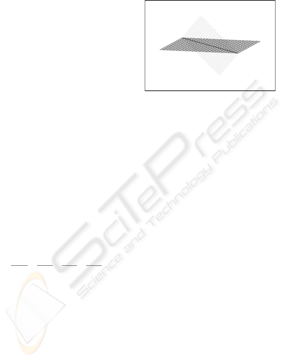
Figure 1 shows two planes intersecting trans-
versely and their intersection line.
Figure 1: Two planar patches intersecting transversely and
their intersection line.
3 GENERALIZING THE
ORIGINAL HEURISTIC
CONSTRAINT
Immediately we see that instead of imposing con-
straint (15) on P(s,t), we could have imposed it on
Q(u,v). That is, we demand instead
u
0
(0) + v
0
(0) = u
0
(1) + v
0
(1) = 2. (28)
After all, it is completely arbitrary which of the two
given surface patches is called P(s,t) and the other
called Q(u,v).
This observation motivates the search for a more
symmetric constraint for determining the parametric
tangents s
0
(a), t
0
(a), u
0
(a), and v
0
(a) at a = 0, 1.
3.1 Other Probable Linear Constraints
To explore the possibilities, we examine condition
(11) carefully and see that it leads to
s(0) + t(0)+ u(0) + v(0) = 0, (29)
s(1) + t(1)+ u(1) + v(1) = 4. (30)
These relations suggest we consider the constraint
σs(a) + τt(a)+ µu(a) + νv(a)
= (σ + τ + µ + ν)a, (31)
or equivalently,
σs
0
(a) + τt
0
(a) + µu
0
(a) + νv
0
(a)
= σ + τ + µ + ν. (32)
Clearly constraint (32) is a generalization of the orig-
inal constraint (15) because the latter is a special case
of the former with
σ = τ = 1, µ = ν = 0. (33)
SURFACE-SURFACE INTERSECTION BY HERMITE INTERPOLATION
25

Consequently, a constraint completely symmetric to
the patches P, Q and the parameters s, t, u, v would
be
σ = τ = µ = ν = 1. (34)
It would be most desirable if being symmetric would
guarantee the best approximation. Unfortunately, this
is not to be so as we shall present a counter example
in Section 4.
The preceding sad remark and the seemingly triv-
ial derivation may cast doubts on the significance of
the generalization. We shall restore confidence by
demonstrating the usefulness of the generalized con-
straint in the following illustration and later discus-
sions. Most significantly, we show in some situa-
tions the generalization produces the exact intersec-
tion with appropriate σ, τ, µ, and ν.
3.2 Illustrating the Generalized
Constraint
The following shows that a twisted cubic curve, which
is the intersection of a quadric cylinder and a cubic
cylinder, can be obtained exactly using the general-
ized constraint (32) with appropriate σ, τ, µ, ν.
Let the quadric cylinder α
2
y = βx
2
and the cubic
cylinder α
3
z = γx
3
be parametrized respectively as
P(s,t) = (αs,βs
2
,γt), 0 ≤ s,t ≤ 1; (35)
Q(u,v) = (αu, βv, γu
3
), 0 ≤ u,v ≤ 1. (36)
Equivalently,
P(s,t) = As + Bs
2
+Ct, (37)
Q(u,v) = Au + Bv +Cu
3
. (38)
where
A = (α,0, 0), B = (0, β, 0),C = (0,0,γ). (39)
The exact intersection C(a) from V
0
= 0 to V
1
=
A + B + C is easily solved analytically and can be
parametrized as
C(a) = (αa, βa
2
,γa
3
), 0 ≤ a ≤ 1. (40)
To find an approximation intersection curve H(a) by
the heuristic we first compute
P
s
= A + 2Bs, P
t
= C, (41)
Q
u
= A + 3Cu
2
, Q
v
= B. (42)
The parametric tangent ratio is
s
0
(a) : t
0
(a) : u
0
(a) : v
0
(a)
= |C,A + 3Cu
2
,B|
: −|A + 2Bs,A + 3Cu
2
,B|
: −|A + 2Bs,C,B|
: |A + 2Bs,C,A + 3Cu
2
|
= 1 : 3u
2
: 1 : 2s (43)
To apply the original constraint on P(s,t), we set
σ = τ = 1, µ = ν = 0 and obtain parametric tangents
s
0
(0),t
0
(0),u
0
(0),v
0
(0) = 2,0, 2, 0; (44)
s
0
(1),t
0
(1),u
0
(1),v
0
(1) =
1
2
,
3
2
,
1
2
,1; (45)
and end-point tangents
T
0
= 2A, T
1
=
A + 2B + 3C
2
. (46)
The resulting approximation cubic Hermite curve is
a
2
¡
a
2
− 3a + 4
¢
A+a
2
(2 − a)B+
a
2
2
(3 − a)C. (47)
To apply the original constraint on Q(u, v), we set
σ = τ = 0, µ = ν = 1 and obtain parametric tangents
s
0
(0),t
0
(0),u
0
(0),v
0
(0) = 2,0, 2, 0; (48)
s
0
(1),t
0
(1),u
0
(1),v
0
(1) =
2
3
,2,
2
3
,
4
3
; (49)
and end-point tangents
T
0
= 2A, T
1
=
2A + 4B + 6C
3
. (50)
The resulting approximation cubic Hermite curve is
a
3
¡
2a
2
− 5a + 6
¢
A +
a
2
3
(5 − 2a)B + a
2
C. (51)
In both the above cases the original constraint did
not produce the exact intersection. But observe that
the intersection is found by setting
s = a,t = a
3
,u = a,v = a
2
. (52)
Thus we may simply set either σ or µ to 1 and the rest
to zero to produce the exact intersection (40). Either
way, the parametric tangents are
s
0
(0),t
0
(0),u
0
(0),v
0
(0) = 1,0, 1, 0; (53)
s
0
(1),t
0
(1),u
0
(1),v
0
(1) = 1,3, 1, 2; (54)
and the end-point tangents are
T
0
= A, T
1
= A + 2B + 3C. (55)
This example reveals that the original constraint may
not produce the exact intersection even when it is a
cubic curve. In contrast, the generalized constraint is
able to produce the exact intersection.
It is worth mentioning that this example does not
contradict Bezout’s theorem despite that the degree
of the intersection curve of a degree two and a degree
three surfaces is three but not six. This is because
here the quadric cylinder and the cubic cylinder has
another intersection line x = w = 0 at infinity of multi-
plicity three. (Here w is the homogenizing coordinate
to enlarge the affine 3-space to a projective 3-space.)
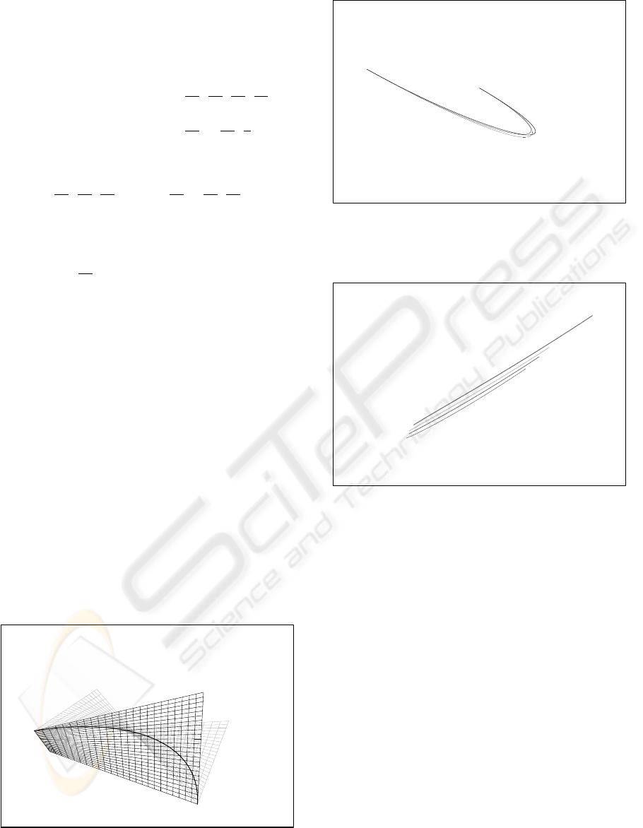
Figure 2 shows the intersection curve, a twisted
cubic curve, and the transversely intersecting quadric
cylinder patch and cubic cylinder patch. Figure 3
shows the exact intersection curve (with σ = 1, τ =
µ = ν = 0 or µ = 1, σ = τ = ν = 0) and the two approx-
imation intersection curves obtained with σ = τ = 1,
µ = ν = 0 and σ = τ = 0, µ = ν = 1.
GRAPP 2008 - International Conference on Computer Graphics Theory and Applications
26
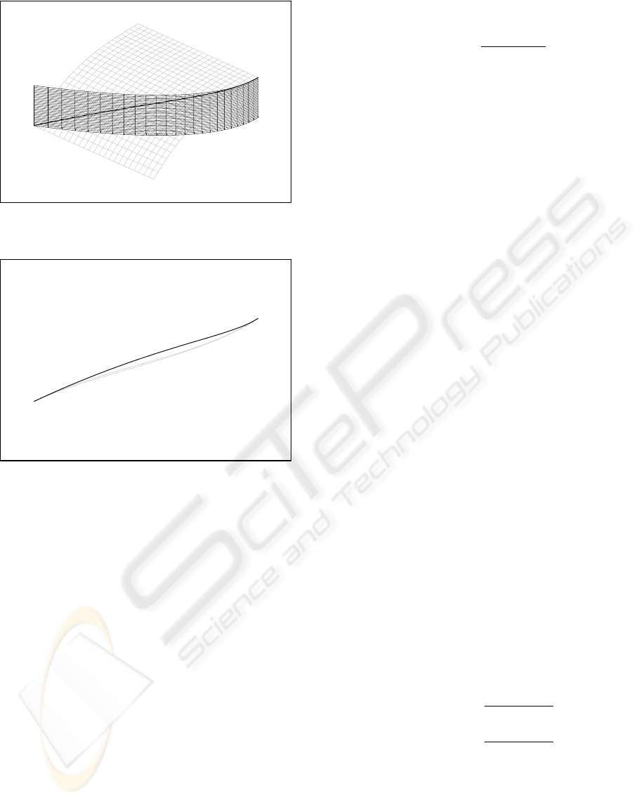
Figure 2: The intersection curve of a quadric cylinder patch
and a cubic cylinder patch.
Figure 3: The two approximation intersection curves (in
thin line) and the exact intersection curve (in thick line) of
a quadric cylinder patch and a cubic cylinder patch.
4 ESTIMATING THE CLOSENESS
OF FIT
By now we see that there are infinitely many gener-
alized constraints for determining the parametric tan-
gents s
0
(a), t
0
(a), u
0
(a), and v
0
(a) at a = 0,1. This
calls for some criteria to assess among constraints
κ which gives a better or best Hermite interpolation
H
κ
(a) to approximate the exact intersection P(s,t) ∩
Q(u,v), ideally parametrized as C(a), 0 ≤ a ≤ 1. For
this purpose we propose a closeness of fit measure-
ment called aggregate square distance.
4.1 The Aggregate Square Distance
Let (s(a),t(a)), (u(a), v(a)) be the pre-images of the
intersection curve C(a), 0 ≤ a ≤ 1, in the parameter
spaces (s,t), (u,v) respectively. That is,
(s(a),t(a)) = P
−1
(C(a)), (56)
(u(a),v(a)) = Q
−1
(C(a)), (57)
where 0 ≤ a ≤ 1. Let |V | be the usual Euclidean norm
for the 1 × 3 vector V ∈ R
3
; that is,
|(x,y, z)| =
p
x
2
+ y
2
+ z
2
. (58)
Consider the integral
I =
Z
1
0
|P(s(a),t(a))− Q(u(a),v(a))|
2
da. (59)
It is obvious that I = 0 if and only if P(s(a),t(a)) =
Q(u(a),v(a)). That is, the integral vanishes if and
only if P(s(a),t(a)) and Q(u(a),v(a)) give the exact
intersection curve C(a).
However, if (s(a),t(a)) and (u(a), v(a)) are only
approximations of the pre-images of the actual inter-
section curve C(a), the integral will give the aggre-
gate square distance of the two approximation curves
C
P
(a) = P(s(a),t(a)) and C
Q
(a) = Q(u(a),v(a)). In
other words, the integral is a measurement of how
close the two approximation curves C
P
(a) and C
Q
(a)
are. It is thus reasonable to extrapolate it to be a mea-
surement of how well H(a) fits C(a). Admittedly this
is a heuristic estimation of the closeness of fit, but em-
pirically it seems to reflect the closeness of fit quite
well as shall be illustrated later.
After adopting the aggregate square distance as a
measurement for the closeness of fit of H(a) to C(a),
our remaining task is to find some approximation pre-
images (s(a),t(a)) and (u(a), v(a)) of C(a) with as
little computing costs as possible.
4.2 Approximating the Pre-Images
Recall that we have already found the parametric tan-
gents s
0
(a), t
0
(a), u
0
(a), and v
0
(a) for a = 0,1. It is
thus with no additional computing costs if we approx-
imate the pre-image of the intersection curve C(a) in
the parameter space (s,t) also with a Hermite cubic
interpolation H
P
(a), by setting the control vertices in
(7) as
V
0
= (0,0), (60)
V
1/3
= V
0
+
(s
0
(0),t
0
(0))
3
, (61)
V
2/3
= V
1
−
(s
0
(1),t
0
(1))
3
, (62)
V
1
= (1,1). (63)
The approximation pre-image H
Q
(a) of the intersec-
tion curve C(a) in the (u,v) space is constructed sim-
ilarly with (s
0
(a),t
0
(a)) replaced by (u
0
(a),v
0
(a)) for
a = 0,1.
To summarize, the intersection curve C(a) and its
pre-images are approximated by three approximation
SURFACE-SURFACE INTERSECTION BY HERMITE INTERPOLATION
27

curves, one in the Euclidean 3-space (x,y,z) and two
in the parameter 2-spaces (s,t) and (u,v):
C(a) = P(s,t) ∩ Q(u,v) ≈ H(a), (64)
P
−1
(C(a)) ≈ H
P
(a), (65)
Q
−1
(C(a)) ≈ H
Q
(a). (66)
Furthermore, we estimate
Z
1
0
|H(a)−C(a)|
2
da (67)
using
Z
1
0
|P(H
P
(a)) − Q(H
Q
(a))|
2
da. (68)
The following theorem affirms the relevance of in-
tegral (68) as a measurement of closeness of fit.
Theorem 1 If integral (68) vanishes and C(a) is cu-
bic in a, then H(a) = C(a).
Proof.
Integral (68) vanishes if and only if P(H
P
(a)) =
Q(H
Q
(a)). But the equality means
P(H
P
(a)) = Q(H
Q
(a)) = P(s,t) ∩ Q(u,v) = C(a).
Thus C(a) and H(a) have the same end-points and
end-point tangents. Consequently they give the same
curve since a parametric cubic curve over [0,1] is
completely determined by its end-points and end-
point tangents. Q.E.D.
We emphasize that H
P
(a) and H
Q
(a) are by-
products from the construction of H(a). It is thus fair
to claim they are available free. Integral (68) can be
integrated numerically with high efficiency because
the integrands are polynomials of low degrees.
4.3 Illustrations
We repeat the tutorial example in (Sederberg and
Nishita, 1991) to illustrate the role of the aggregate
square distance in identifying a constraint for a closer-
fitting approximation H(a).
Consider two bilinear patches
P(s,t) =
1
∑
i, j=0
P
i j
(1 − s)
1−i
s
i
(1 −t)
1− j
t
j
, (69)
and
Q(u,v) =
1
∑
i, j=0
Q
i j
(1 − u)
1−i
u
i
(1 − v)
1− j
v
j
, (70)
where
P
00
,P
10
,P
01
,P
11
=
[0,0, 0] , [0, 1, 4],[3,3,0],[4,0, 4] ; (71)
and
Q
00
,Q
10
,Q
01
,Q
11
=
[0,0, 0] , [0, 4, 4],[4,2,0],[4,0, 4] . (72)
The example in (Sederberg and Nishita, 1991)
used the Sederberg-Nishita constraint on P(s,t) by
setting
σ = τ = 1, µ = ν = 0, (73)
and obtained the parametric tangents
s
0
(0),t
0
(0),u
0
(0),v
0
(0) =
2
3
,
4
3
,
2
3
,1; (74)
s
0
(1),t
0
(1),u
0
(1),v
0
(1) = 2,0, 2,
1
2
. (75)
The resulting end-point tangents were
T
0
=
·
4,
14
3
,
8
3
¸
,T
1
= [2,−6, 8] , (76)
and thus
H
1100
(a) =
−2a(a
2
− a − 2)
−
2a
3
(2a
2
+ 5a − 7)
4a
3
(2a
2
− a + 2)
T
. (77)
The aggregate square distance for this approximation
is
ρ
1100
= 0.0053561. (78)
Now we try using the Sederberg-Nishita con-
straint on Q(u,v) instead of P(s,t); that is, we set
σ = τ = 0, µ = ν = 1. (79)
The parametric tangents are
s
0
(0),t
0
(0),u
0
(0),v
0
(0) =
4
5
,
8
5
,
4
5
,
6
5
; (80)
s
0
(1),t
0
(1),u
0
(1),v
0
(1) =
8
5
,0,
8
5
,
2
5
. (81)
The resulting end-point tangents are
T
0
=
·
24
5
,
28
5
,
16
5
¸
,T
1
=
·
8
5
,−
24
5
,
32
5
¸
, (82)
and thus
H
0011
(a) =
4a
5
−(2a
2
− a − 6)
(a
2
− 8a + 7)
(2a
2
− a + 4)
T
. (83)
The aggregate square distance for this approximation
is
ρ
0011
= 0.00032996. (84)
Since ρ
0011
is much smaller than ρ
1100
, we expect
H
0011
(a) to be a closer fit than H
1100
(a). This is
found to be so by visually inspecting a plot of P(s,t),
Q(u,v), H
1100
(a), and H
0011
(a).
GRAPP 2008 - International Conference on Computer Graphics Theory and Applications
28
Finally we assess the performance of the symmetric
constraint
σ = τ = µ = ν = 1. (85)
The parametric tangents are
s
0
(0),t
0
(0),u
0
(0),v
0
(0) =
8
11
,
16
11
,
8
11
,
12
11
;(86)
s
0
(1),t
0
(1),u
0
(1),v
0
(1) =
16
9
,0,
16
9
,
4
9
. (87)
The resulting end-point tangents are
T
0
=
·
48
11
,
56
11
,
32
11
¸
,T
1
=
·
16
9
,−
16
3
,
64
9
¸
, (88)
and thus
H
1111
(a) =
4a
99
−(46a
2
− 37a − 108)
−6(a
2
+ 20a − 21)
(50a
2
− 23a + 72)
T
. (89)
The aggregate square distance for this approximation
is
ρ
1111
= 0.0016125. (90)
We observe that
ρ
0011
< ρ
1111
< ρ
1100
. (91)
With a visual inspection of a plot of P(s,t), Q(u,v),
H
0011
(a), H
1111
(a), and H
1100
(a), it is satisfying to
see that the aggregate square distance does faithfully
reflect the closeness of fit.
Figure 4 shows the bilinear patches and their
intersection curve. Figure 5 and figure 6 shows
the three approximation intersection curves H
1100
(a),
H
0011
(a), H
1111
(a) and the actual intersection curve
C(a). Visually we ascertain that H
0011
(a) fits best
while H
1100
(a) fits worst and H
1111
(a) is somewhere
in between. This is consistent with the prediction of
their aggregate square distances.
Figure 4: The bilinear patches P(s,t), Q(u, v), and their in-
tersection C(a).
Figure 5: The cubic Hermite curves H
1100
(a), H
1111
(a),
H
0011
(a) and the exact intersection curve C(a), 0 ≤ a ≤ 1,
for the bilinear patches.
Figure 6: The top curve is the exact intersection curve. In
increasing distance from the top curve are the curves ob-
tained with constraints σ = τ = 0,µ = ν = 1; σ = τ = µ =
ν = 1; σ = τ = 1, µ = ν = 0 respectively. All curves are
plotted from 0.3 to 0.7 to magnify their separation.
5 OBSERVATIONS AND
SPECULATIONS
From the above discussions, we realize that the
approximation cubic Hermite curves H
1100
(a) and
H
0011
(a) fit the intersection curve C(a) with differ-
ent accuracy and one can be a much better fit than
the other. The winner can be determined by compar-
ing their aggregate square distances ρ
1100
and ρ
0011
,
which can be computed efficiently with little addi-
tional computing costs.
Intuitively, we would expect the approximation
cubic Hermite curve H
1111
(a), in terms of accuracy,
to be worst than the best of H
1100
(a), H
0011
(a) but
better than the worst of them. This speculation is sup-
ported by our example. It would be very helpful in
establishing the applicability of the aggregate square
SURFACE-SURFACE INTERSECTION BY HERMITE INTERPOLATION
29

distance measurement if this guess can be established
as a fact with some proof.
We have shown that when the surface patches are
planar, the Sederberg-Nishita heuristic produces the
exact intersection line with a proper parametrization,
despite the use of a cubic Hermite interpolation. This
has greatly enhanced the credibility of the Sederberg-
Nishita constraint used in the heuristic. It would be
interesting in theory and useful in practice if more
cases can be discovered in which the cubic Hermite
curve is the actual intersection curve rather than just
an approximation. It would be even better if some
sufficient or necessary conditions can be laid down
under which the generalized constraint produces the
exact intersection curve.
In this paper we only exploit polynomial cubic
Hermite interpolation. It should be a worthwhile ef-
fort to explore the use of rational Hermite interpola-
tion (Goldman, 2003) for approximating the intersec-
tion curve of two surface patches. Note that some ra-
tional curves, such as circular arcs, do not have poly-
nomial parametrization.
6 CONCLUSIONS
We first reviewed a quick heuristic originally pro-
posed by Sederberg and Nishita. The heuristic finds a
cubic Hermite interpolation curve that approximates
the intersection of two rationally parametrized sur-
face patches when they intersect transversely. The
power of the heuristic was established empirically in
(Sederberg and Nishita, 1991). We further enhanced
its credibility by showing that when the surfaces are
planes the heuristic actually produces the exact inter-
section line parametrized properly.
The heuristic utilizes a constraint to decide the
parametric tangents in order to compute the Hermite
interpolation. The constraint is arbitrarily applied to
one of the two surfaces in the heuristic. We proposed
that the constraint should be applied to both surfaces
individually thus producing two approximating cubic
Hermite curves. The better-fitting one should then
be used. The assessment is based on their aggregate
square distances which can be easily evaluated. An
example was given to illustrate that much improve-
ment in accuracy could be achieved. All this was done
with very little additional computing costs, as it was
crucial not to sacrifice speed of the heuristic to attain
better accuracy.
This way of applying the constraint can be consid-
ered as special cases of deploying of what we called
the generalized constraint. We showed that there are
situations in which the generalized constraint could
produce the exact intersection curve but the original
constrain could not.
We also discussed some interesting open problems
with this new perspective on the constraint.
REFERENCES
Cox, D., John, L., and Donal, O. (1998). Using Algebraic
Geometry. Springer, New York.
de Figueiredo, L. H. (1996). Surface intersection us-
ing affine arithmetic. Proceedings of Graphics Inter-
face’96.
Fulton, W. (1969). Algebraic Curves: An Introduction to Al-
gebraic Geometry. W. A. Benjamin, Inc., New York.
Goldman, R. N. (2003). Pyramid Algorithms : A dynamic
programming approach to curves and surfaces for ge-
ometric modeling. Morgan Kaufmann, San Francisco.
Katz, S. and Sederberg, T. W. (1988). Genus of the intersec-
tion curve of two rational surface patches. Computer
Aided Geometric Design, 5:253–258.
Sederberg, T. W. (1986). Improperly parametrized rational
curves. Computer Aided Geometric Design, 3:1:67–
75.
Sederberg, T. W. and Nishita, T. (1991). Geometric hermite
approximation of surface patch intersection curves.
Computer Aided Geometric Design, 8:97–114.
Song, X., Sederberg, T., Zheng, J., Farouki, R., and Hass, J.
(2004). Linear perturbation methods for topologically
consistent representations of free-form surface inter-
sections. Computer Aided Geometric Design, 21:303–
319.
GRAPP 2008 - International Conference on Computer Graphics Theory and Applications
30
