VISUALIZING MULTIPLE SCALAR FIELDS ON A SURFACE

Mohammed Mostefa Mesmoudi

Institut Universitaire de Formation des Maˆıtres de Cr´eteil, 12 rue George Enesco, 94046 Cr´eteil, France

Leila De Floriani, Paola Magillo

Department of Computer Science and Information Science, University of Genova, Via Dodecaneso, 35 -16146 Genova, Italy

Keywords:

3D Visualization, geometric modeling, multivariate scalar ﬁelds, offsetting.

Abstract:

We present a new technique for the simultaneous visualization of an arbitrary number of scalar ﬁelds deﬁned

on a surface. The technique is called Generalized Atmosphere Upper Bound Level (GAUBL), since it is an

evolution of our previous AUBL technique, that allowed for the visualization of a single scalar ﬁeld. The

generalized AUBL can highlight the dependencies and interactions between many scalar ﬁelds, and can handle

a multi-valued scalar ﬁeld as a special case. We have implemented the GAUBL into a visualization tool that

handles triangle-based surface models, and we show here some experimental results.

1 INTRODUCTION

In many applicationsof computergraphics (e.g., med-

ical imagery, visual data mining) the visualizationof a

scalar ﬁeld representing some data relative to a three-

dimensional shape is a basic tool to explore and un-

derstand the behaviorof the ﬁeld. Several scalar ﬁelds

may be interesting to be studied simultaneously, to

highlight their dependencies and their mutual inﬂu-

ence. For example, in medical imagery, oxygen rate

and sugar rate can be visualized together to study the

brain surface activity. Unfortunately, human percep-

tion is limited to three dimensions and the visualiza-

tion of those scalar ﬁelds needs additional indepen-

dent directions to be achieved. To avoid this obstacle,

we need to ﬁnd a natural way to embed these multi-

dimensional data in the Euclidean space R

so that

the result still has some meaningful interpretation, es-

pecially for comparison purposes. Here, we propose

a visualization technique that allows this embedding

and thus gives us the opportunity to explore and study

multi-valued scalar ﬁelds deﬁned on the same sur-

face. The basic idea is to convert the scalar ﬁelds into

a sequence of vector ﬁelds on the surface and then

display a surface for each vector ﬁeld according to

some constraints. We call the new visualization tech-

nique Generalized AUBL (GAUBL), since it general-

izes to multi-dimensional scalar ﬁelds the AUBL (At-

mosphere Upper Bound Level) technique introduced

in (Mesmoudi et al., 2007). This latter allows the

3D visualization of just one scalar ﬁeld deﬁned over a

surface embedded in the three-dimensional Euclidean

space. The generalized AUBL technique is easily

adapted to handle discrete scalar ﬁelds deﬁned over

triangulated surfaces. We present here an interactive

visualization tool that implements the GAUBL tech-

nique for triangle meshes. We use such tool to il-

lustrate the results of the GAUBL visualization tech-

nique. The remainder of the paper is organized as

follows. In Section 2, we review related work. In

Sections 3, we brieﬂy review the AUBL visualization

technique. In Section4, we introduce the GAUBL vi-

sualization technique that generalizes AUBL to visu-

alizing several scalar ﬁelds. In Section 5, we present

the visualization tool implementing the GAUBL tech-

nique for discrete scalar ﬁelds deﬁned on triangulated

surfaces, and some results. In the last Section, we

draw some concluding remarks.

2 RELATED WORK

To represent multi-dimensional data in the three di-

mensional space, we need to reduce their dimension-

ality without loosing important information. Geo-

138

Mostefa Mesmoudi M., De Floriani L. and Magillo P. (2008).

VISUALIZING MULTIPLE SCALAR FIELDS ON A SURFACE.

In Proceedings of the Third International Conference on Computer Graphics Theory and Applications, pages 138-142

DOI: 10.5220/0001097201380142

 SciTePress

metric projection techniques allow meaningful visu-

alization of multi-dimensional data. Some of them

are statistically based techniques (Huber, 1985). Par-

allel coordinates techniques (Inselberg, 1985) repre-

sent attributes as parallel lines in the two-dimensional

space. Hierarchical techniques use a partitioning of

the space into subspaces. In stacking techniques, the

space is partitioned into 2D subspaces that are stacked

in a recursive way (Blanc et al., 1990). The worlds-

within-worlds technique partitions the 3D space into

nested subspaces: three attributes are selected and vi-

sualized through a 3D surface, then, for any point on

the surface selected by the user, three other attributes

are visualized in the same manner (Feiner and Besh-

ers, 1990). When some attributes are functions of two

or three dependent parameters (like in terrain model-

ing, image processing, medical imagery), the graph-

ical representation of these attributes has more sense

if it can be represented in the ambient space by a sur-

face. The AUBL technique developed in (Mesmoudi

et al., 2007) allows the 3D visualization of a scalar

ﬁeld deﬁned over a surface embedded in the 3D Eu-

clidean space. This technique when applied to a con-

stant function is known as offsetting (Rossignac and

Requicha, 1985; Frisken et al., 2000; Cohen et al.,

1996). In (Taylor, 2002; Kirby et al., 1999; Craw-

ﬁs and Allison, 1991), techniques to represent multi-

ple scalar ﬁelds (at most four ﬁelds) on the same sur-

face have been proposed. These techniques combine

colors, contour lines, spot noise texture generation,

reaction-diffusion texture generation, surface albedo,

data-driven spots and oriented slivers.

3 THE AUBL VISUALIZATION

TECHNIQUE

Two-dimensional manifolds (without boundary) are

(smooth) surfaces that are locally diffeomorphic to

discs in R

. At each point p of a surface S, the tangent

plane T

S is deﬁned and a unit normal vector

−→

to S

at point p can be drawn. This latter correspondence is

called the Gauss map. Vector

−→

with an orthonormal

basis of T

S generates a mobile orthonormal frame of

the Euclidean three-dimensional space R

whose ori-

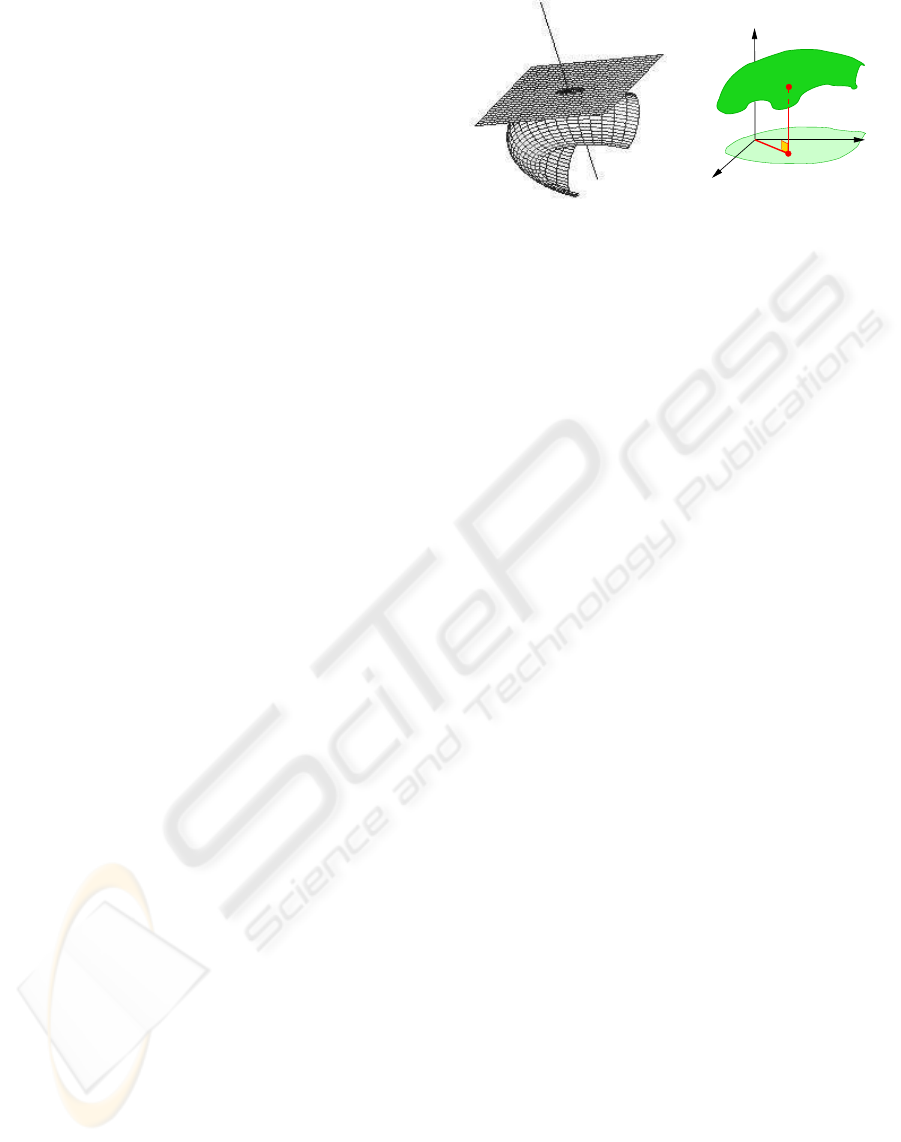
gin is located at point p (see Figure 1(a)). The key

idea of the AUBL visualization technique comes from

the graphical representation of 2D scalar ﬁelds. The

graphical representation of a scalar ﬁeld g on a two-

dimensional domain D

∼

D×0 is a surface embedded

in R

such that the height of each point on the surface

corresponds to the value of g at this point and if the

frame is orthonormal then the distance of the point to

the Oxy-plane is equal to the absolute value of g at

g(D)

g(m)

(a) (b)

Figure 1: (a) A surface with its tangent plane and normal

vectorial space at a point. (b) Graphical representation of a

function g over a domain D ⊂ R

this point (see Figure 1(b)). By generalizing this idea,

we can give a graphical representation of 3D scalar

ﬁelds.

Deﬁnition 1 Let

−→

be the unit normal vector of S at

point p. The graphical representation of the scalar

ﬁeld f over S is the surface S ⊂ R

deﬁned by the

vector ﬁeld

f(p) := p+ f(p)

−→

, i.e.,

S = {p + f(p)

−→

: p ∈ S} (1)

Note that vector

−−−→

f(p) is normal to S at p and

−−−→

f(p) k=| f(p) |.

The graphical representation of function f deﬁnes an

atmosphere layer over surface S. The thickness of

the layer is given by the function values. In (Mes-

moudi et al., 2007), we have deﬁned graphical opera-

tions which can be used to better analyze the shape of

the surface and thus the properties of the ﬁeld. Scal-

ing multiplies the ﬁeld vector value through a factor;

inﬂation and deﬂation translate

f(p) in direction of

the normal vector

−→

by a constant positive and nega-

tive value, respectively. Details can be found in (Mes-

moudi et al., 2007).

Deﬁnition 2 Under such assumptions, we call the

graphical representation S of f, the atmosphere up-

per bound layer (AUBL) of the pair (S, f).

In Figure 2, we illustrate the above situation for the

unit sphere x

+ y

+ z

= 1 with an atmosphere cor-

responding to the function f(x, y, z) = x

− y

− 1.

4 THE GENERALIZED AUBL

TECHNIQUE

The main idea in generalizing the AUBL visualization

technique comes from the fact that the AUBL tech-

nique gives a vector ﬁeld



−−−→

f(p)



p∈S

over surface S.

VISUALIZING MULTIPLE SCALAR FIELDS ON A SURFACE

139

(a) (b)

Figure 2: (a) A cross section of the unit sphere with an at-

mosphere deﬁned by function f(x, y, z) = x

− y

− 1. (b)

Visualization of S corresponding to

We use this idea to generate a vector ﬁeld over S for

any number of functions deﬁned on S. We will show

that successive vector ﬁelds can be deﬁned depending

on the number of functions. Assume that two scalar

ﬁelds f and g are deﬁned simultaneously on S. AUBL

visualization technique is used to visualize function f

as surface S . To visualize function g with f, a col-

oring map c is deﬁned on the image Im(g). Then a

vector function ˜g can be deﬁned as follows: for each

point p ∈ S we associate the pair (

f(p), c(g(p))). Fi-

nally, functions (f, g) are visualized as a colored sur-

face, that we denote C S to distinguish it from S . Fig-

ure 3(a) gives an example of two functions f and g

deﬁned on the unit sphere S

. Let now f, g and h be

(f(m), g(m), h(m))

(a) (b)

Figure 3: (a) Visualization of two functions f (x, y, z) =

and g(x, y, z) = z

deﬁned over the unit sphere. Func-

tion f is represented as a surface containing the unit sphere

in its interior, and g is represented by a coloring map where

white and magenta correspond to low and high ﬁeld values,

respectively. (b) Graphical representation of three scalar

ﬁelds over a surface S in R

three scalar ﬁelds deﬁned on surface S. For each point

p ∈ S, we deﬁne a vector

−→

= ( f(p), g(p), h(p)).

This gives a vector ﬁeld



−→



p∈S

over S (see Figure

3(b)). We deﬁne surface S := {p +

−→

: p ∈ S} as

the graphical representation of scalar ﬁelds f, g and

h over S. The direction and the intensity of each vec-

tor is inﬂuenced by the values of the three functions

f, g and h. Thus, interactions among these func-

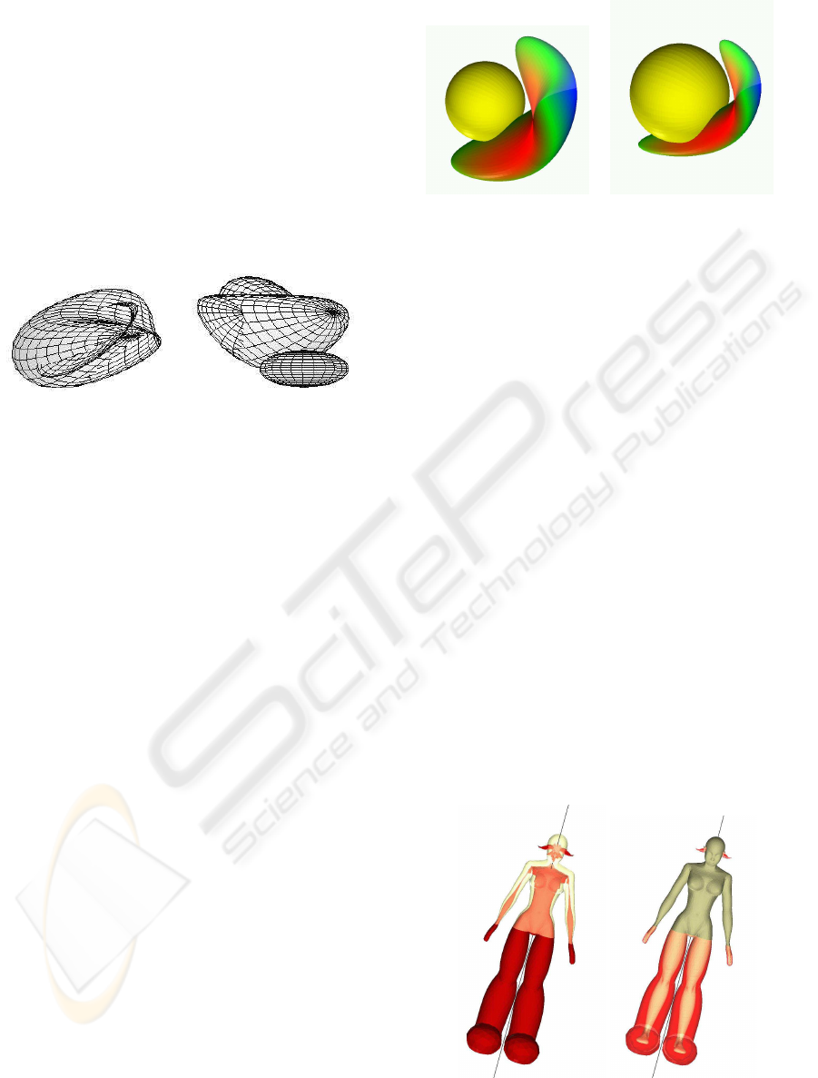
tions can be seen (see Figure 4). For four scalar

Figure 4: Visualization of three functions f(x, y, z) = x

, g(x, y, z) = z

and h(x, y, z) = y− z deﬁned over the unit

sphere, from two different points of view. Functions f , g, h

are presented as the surface of a vector ﬁeld ( f, g, h).

ﬁelds f, g, h and k, we embed surface S in R

S ≈ S

′

:= {(x, y, z, 0) : (x, y, z) ∈ S}. For each point

p ∈ S we deﬁne a vector

−→

′

= ( f(p), g(p), h(p), k(p)).

Vectors



−→

′



p∈S

form a vector ﬁeld over S

′

. Visual-

ization of scalar ﬁelds f, g, h and k can be achieved in

by constructing a new surface S

′

:= {(p, 0) +

−→

′

p ∈ S} = {(x

+ f(p), y

+ g(p), z

+ h(p), k(p))}.

Equivalently, S

′

can be seen as a surface S” := {(x

f(p), y

+ g(p), z

+ h(p)) : p ∈ S} in R

endowed

with a scalar ﬁeld k. Function k can be seen as a color-

ing function of surface S”. Another way to represent

function k is to use the AUBL visualization technique

that permits to deﬁne a surface S ” ⊂ R

associated

with the pair (S”, k). We deﬁne thus (S”, S ”) to be the

graphical representation of scalar ﬁelds f, g, h and k.

Now, the generalization to ﬁve scalar ﬁelds can

be done as for the case of two scalar ﬁelds. We

represent the fourth scalar ﬁeld by the AUBL tech-

nique as a surface S ” and the ﬁfth scalar ﬁeld by

a coloring function over surface S ”. The colored

surface C S ” with S” give a graphical representation

of the all ﬁve scalar ﬁelds (see Figure 5). For six

(a) (b)

Figure 5: Visualization of ﬁve functions f(x, y, z) = x

g(x, y, z) = z

, h(x, y, z) = 2y− z + 3,k(p) = z and l(p) = x

deﬁned over the unit sphere S

. (a) Surfaces S

, S” and S ”.

(b) The coloring function l is represented in C S ”.

scalar ﬁelds f, g, h, k, l and m, we shift surface

S to R

to get a surface S ≈ S

′

:= {(x, y, z, 0, 0, 0) :

(x, y, z) ∈ S}. Then for each point p ∈ S we de-

ﬁne a vector

−→

′

= ( f(p), g(p), h(p), k(p), l(p), m(p)).

Vectors



−→

′



p∈S

form a vector ﬁeld that traverses

GRAPP 2008 - International Conference on Computer Graphics Theory and Applications

140

over S

′

. Visualization of scalar ﬁelds f, g, h, k, l

and m can be achieved in R

by constructing surface

′

:= {(p, 0, 0, 0) +

−→

′

: p ∈ S} = {(x

+ f(p), y

g(p), z

+ h(p), k(p), l(p), m(p))}. Equivalently, S

′

can be seen as a surface S” := {(x

+ f(p), y

g(p), z

+ h(p)) : p ∈ S} embedded in R

with a vec-

tor ﬁeld deﬁned by vectors

−−→

V”

= (k(p), l(p), m(p)).

Then as for three scalar ﬁelds we can construct a sur-

face S ” deﬁned by vectors

−−→

V”

. The visualization of

all scalar ﬁelds f, g, h, k, l and m is hence given

by two surfaces (S”, S ”) as in Figure 6. Following

(a) (b)

Figure 6: Visualization of six functions f (x, y, z) = x

+ y

g(x, y, z) = z

, h(x, y, z) = 2y − z + 3,k(p) = z, and m(p) =

−y

. Functions f, g and h form a ﬁrst vector ﬁeld S

′

over

. Then function k, l and m form a second vector ﬁeld over

′

. (a) Surfaces S

′

and S ”. (b) Surfaces S

, S

′

and S ”.

the previous reasoning, we can extend (modulo 3) the

above visualization techniques to n scalar ﬁelds de-

ﬁned over surface S. The AUBL technique, the color-

ing technique and thevector ﬂowtechniqueforma ba-

sis of the visualization techniques that can be used to-

gether, or separately, following the rank of n (mod 3).

This extension gives a hierarchical representation of

scalar ﬁelds as described in the worlds-with-worlds

data mining representation technique (see Section 2

above).

5 EXPERIMENTAL RESULTS

Our GAUBL tool allows for the visualization of up to

four different scalar ﬁelds deﬁned on a triangulated

surface. It is implemented in C with the OpenGL

graphical library and has a very simple user interface

developed with Glut. The surface is given as a tri-

angle mesh in indexed format (each vertex as three

coordinates, each triangle as three vertex indexes). A

scalar ﬁeld can be provided in two forms: an explicit

list of ﬁeld values at the mesh vertices (e.g., sampled

values of temperature, pressure etc.), or a mathemat-

ical formula to compute such values. Visualization

adapts to the current number of loaded scalar ﬁelds,

by selecting the appropriate GAUBL technique. Ad-

ditional inputs are represented by coloring functions

Figure 7: The sphere and four ﬁelds, with two different mul-

tiplication factors.

to map ﬁeld values to color values speciﬁed in the

red-green-blue (RGB) format. The user can interac-

tively set parameters, as the translation factor for in-

ﬂation / deﬂation, the multiplicative factor for scaling,

the coloring function, surface and background colors,

transparency effects, and, of course, he can rotate, pan

and zoom the entire scene. Figure 7 shows the unite

sphere along with the colored mesh representing four

scalar ﬁelds: f (p) = x, g(p) = y − z, h(p) = x

+ y

and k(p) = x, the last one rendered with a coloring

function going from red to blue through green. Figure

8 shows a mesh representing a girl and a ﬁeld equal

to f(p) = z. In Figure 9 the same mesh is associ-

ated with a scalar ﬁeld that simulates fattening of the

central part of the body, through a gaussian formula.

The ﬁgure shows the original surface and two fattened

versions, with different multiplication factors. Figure

10 shows a terrain with two scalar ﬁelds, where the

ﬁrst one (giving the surface) is constant and the sec-

ond one (rendered as color scale) is g(p) = z. Inﬂa-

tion and deﬂation correspond here to a version of the

same terrain after deposit of material (e.g. calcium

carbonate on the bottom of a lake in a cavern) or after

erosion, respectively.

Figure 8: Girl surface with one ﬁeld f(p) = z.

VISUALIZING MULTIPLE SCALAR FIELDS ON A SURFACE

141

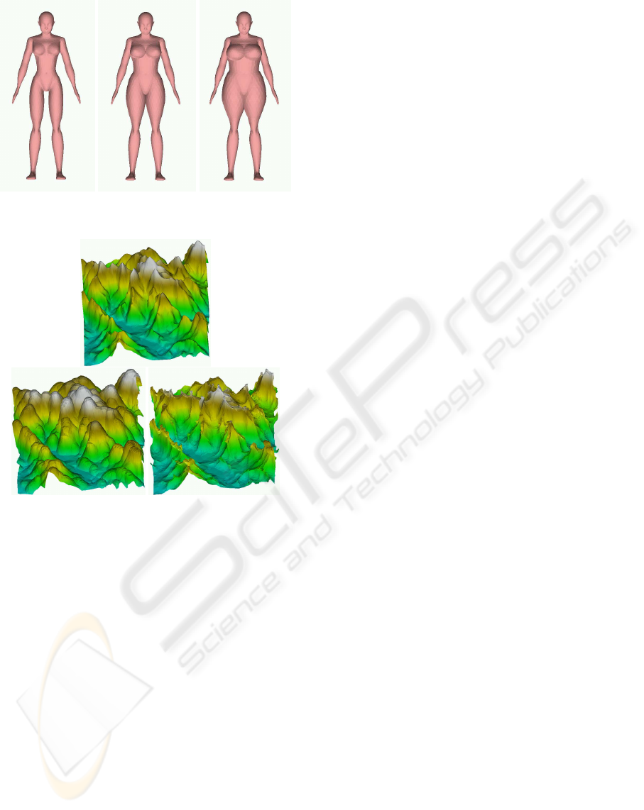
Figure 9: Girl surface with different multiplication factors.

Figure 10: A terrain and its inﬂated and deﬂated versions.

6 CONCLUDING REMARKS

We have presented the GAUBL visualization tech-

nique that allows displaying any number of scalar

ﬁelds deﬁned on a surface, in the form of another

(possibly colored) surface embedded in 3D space. In

our ongoing work, we will improve our visualization

tool with new functionalities, such as showing alge-

braic information at a clicked point on the surface

(vector length, direction, position with respect to the

normal vector of the original surface,...). Moreover,

we plan to combine this visualization technique with

a mesh-based multi-resolution representation to allow

selective and adaptive offsetting of a surface.

ACKNOWLEDGEMENTS

This work has been partially supported by the Eu-

ropean Network of Excellence AIM@SHAPE un-

der contract number 506766, by the National Sci-

ence Foundation under grant CCF-0541032, by the

MIUR-FIRB project SHALOM under contract num-

ber RBIN04HWR8 and by the MIUR-PRIN project

on ”Multi-resolution modeling of scalar ﬁelds and

digital shapes”.

REFERENCES

Blanc, J. L., Ward, M., and Wittels, N. (1990). Exploring

n-dimensional databases. In Visualization’90, pages

230–238, San Fransisco, CA.

Cohen, L., Varshney, A., Manocha, D., Turk, G., Weber,

H., Agarwal, P., Brooks, P., and Wright, W. (1996).

Simpliﬁcation envelopes. In Proc. ACM SIGGRAPH,

pages 119–128.

Crawﬁs, R. and Allison, M. (1991). A scientiﬁc visual-

ization synthetizer. In Proc. IEEE Viaualization’91,

IEEE CS Press, Los Alamitos, CA.

Feiner, S. and Beshers, C. (1990). World within world

: Metaphors for exploring n-dimensional virtual

worlds. In Proceedings UIST, pages 76–83.

Frisken, S. F., Perry, R. N., Rockwood, A. P., and Jones,

T. R. (2000). Adaptively sampled distance ﬁelds: A

general representation of shape for computer graphics.

Technical report, Mitsubishi Electric Research Labo-

ratories, Cambridge Research Center. TR2000-15.

Huber, P. J. (1985). Projection pusuit. Annals of Statistics,

13(2):435–474.

Inselberg, A. (1985). The plane with parallel coordinates.

Special Issue On Computational Geometry, The Vi-

sual Computer, 1:69–97.

Kirby, R., Marmanis, H., and Laidlaw, D. (1999). Visual-

izing multivalued data fron 2d incompressible ﬂows

using concepts from painting. In Proc. IEEE Visual-

ization’99, IEEE CS Press, Los Alamitos, CA, pages

333–340.

Mesmoudi, M., Floriani, L. D., and Rosso, P. (2007). Theo-

retical foundations of 3d scalar ﬁelds visualization. In

Proceedings of Special Sesssions International con-

ference on computer vision theory and application,

pages 69–77, Barcelona Spain. INSTICC Press.

Rossignac, J. and Requicha, A. (1985). Offsetting oper-

ations in solid modeling. Computer Aided Design,

3(2):129–148.

Taylor, R. (2002). Visualizing multiple ﬁelds on the same

surface. Visualization Viewpoints, IEEE Computer

Graphics and applications, May/June:6–11.

GRAPP 2008 - International Conference on Computer Graphics Theory and Applications

142